LitPop class#
Introduction#
LitPop is an Exposures-type class. It is used to initiate gridded exposure data with estimates of either asset value, economic activity or population based on nightlight intensity and population count data.
Background#
The modeling of economic disaster risk on a global scale requires high-resolution maps of exposed asset values. We have developed a generic and scalable method to downscale national asset value estimates proportional to a combination of nightlight intensity (“Lit”) and population data (“Pop”).
Asset exposure value is disaggregated to the grid points proportionally to \(Lit^m Pop^n\), computed at each grid cell:
\(Lit^mPop^n = Lit^m * Pop^n\), with \(exponents = [m, n] \in \mathbb{R}^{+}\) (Default values are \(m=n=1\)).
For more information please refer to the related publication (https://doi.org/10.5194/essd-12-817-2020) and data archive (https://doi.org/10.3929/ethz-b-000331316).
How to cite: Eberenz, S., Stocker, D., Röösli, T., and Bresch, D. N.: Asset exposure data for global physical risk assessment, Earth Syst. Sci. Data, 12, 817–833, https://doi.org/10.5194/essd-12-817-2020, 2020.
Input data#
Note: All required data except for the population data from Gridded Population of the World (GPW) is downloaded automatically when an LitPop.set_* method is called.
Warning: Processing the data for the first time can take up huge amounts of RAM (>10 GB), depending on country or region size. Consider using the wrapper function of the data API to download readily computed LitPop exposure data for default values (\(n = m = 1\)) on demand.
Nightlight intensity#
Black Marble annual composite of the VIIRS day-night band (Grayscale) at 15 arcsec resolution is downloaded from the NASA Earth Observatory: https://earthobservatory.nasa.gov/Features/NightLights (available for 2012 and 2016 at 15 arcsec resolution (~500m)). The first time a nightlight image is used, it is downloaded and stored locally. This might take some time.
Population count#
Gridded Population of the World (GPW), v4: Population Count, v4.10, v4.11 or later versions (2000, 2005, 2010, 2015, 2020), available from http://sedac.ciesin.columbia.edu/data/collection/gpw-v4/sets/browse.
The GPW file of the year closest to the requested year (reference_year) is required.
To download GPW data a (free) login for the NASA SEDAC website is required.
Direct download links are avilable, also for older versions, i.e.:
v4.11: http://sedac.ciesin.columbia.edu/downloads/data/gpw-v4/gpw-v4-population-count-rev11/gpw-v4-population-count-rev11_2015_30_sec_tif.zip
v4.10: http://sedac.ciesin.columbia.edu/downloads/data/gpw-v4/gpw-v4-population-count-rev10/gpw-v4-population-count-rev10_2015_30_sec_tif.zip,
Overview over all versions of GPW v.4: https://beta.sedac.ciesin.columbia.edu/data/collection/gpw-v4/sets/browse
The population data from GWP needs to be downloaded manually as TIFF from this site and placed in the SYSTEM_DIR folder of your climada installation.
Downloading existing LitPop asset exposure data#
The easiest way to download existing data is using the wrapper function of the data API.
Readily computed LitPop asset exposure data based on \(Lit^1Pop^1\) for 224 countries, distributing produced capital / non-financial wealth of 2014 at a resolution of 30 arcsec can also be downloaded from the ETH Research Repository: https://doi.org/10.3929/ethz-b-000331316. The dataset contains gridded data for more than 200 countries as CSV files.
Attributes#
The LitPop class inherits from Exposures.
It adds the following attributes:
    exponents : Defining powers (m, n) with which nightlights and population go into Lit**m * Pop**n.
    fin_mode : Socio-economic indicator to be used as total asset value for disaggregation.
    gpw_version : Version number of GPW population data, e.g. 11 for v4.11
fin_mode#
The choice of fin_mode is crucial. Implemented choices are:
'pc': produced capital (Source: World Bank), incl. manufactured or built assets such as machinery, equipment, and physical structures. The pc-data is stored in the subfolder data/system/Wealth-Accounts_CSV/. Source: https://datacatalog.worldbank.org/dataset/wealth-accounting'pop': population count (source: GPW, same as gridded population)'gdp': gross-domestic product (Source: World Bank)'income_group': gdp multiplied by country’s income group+1'nfw': non-financial household wealth (Source: Credit Suisse)'tw': total household wealth (Source: Credit Suisse)'norm': normalized, total value of country or region is 1.'none': None – LitPop per pixel is returned unchanged
Regarding the GDP (nominal GDP at current USD) and income group values, they are obtained from the World Bank using the pandas-datareader API. If a value is missing, the value of the closest year is considered. When no values are provided from the World Bank, we use the Natural Earth repository values.
Key Methods#
from_countries: set exposure for one or more countries, see sectionfrom_countriesbelow.from_nightlight_intensity: wrapper aroundfrom_countriesandfrom_shapeto load nightlight data to exposure.from_population: wrapper aroundfrom_countriesandfrom_shape_populationto load pure population data to exposure. This can be used to initiate a population exposure set.from_shape_and_countries: given a shape and a list of countries, exposure is initiated for the countries and then cropped to the shape. See section Set custom shapes below.from_shape: given any shape or geometry and an estimate of total values, exposure is initiated for the shape directly. See section Set custom shapes below.
# Import class LitPop:
from climada.entity import LitPop
from_countries#
In the following, we will create exposure data sets and plots for a variety of countries, comparing different settings.
Default Settings#
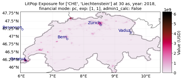
Per default, the exposure entity was initiated using the default parameters, i.e. a resolution of 30 arcsec, produced capital ‘pc’ as total asset value and using the exponents \((1, 1)\).
# Initiate a default LitPop exposure entity for Switzerland and Liechtenstein (ISO3-Codes 'CHE' and 'LIE'):
try:
    exp = LitPop.from_countries(
        ["CHE", "Liechtenstein"]
    )  # you can provide either single countries or a list of countries
except FileExistsError as err:
    print(
        "Reason for error: The GPW population data has not been downloaded, c.f. section 'Input data' above."
    )
    raise err
exp.plot_scatter()

# Note that `exp.gdf['region_id']` is a number identifying each country:
print("\n Region IDs (`region_id`) in this exposure:")
print(exp.gdf["region_id"].unique())
2021-10-19 17:03:20,108 - climada.entity.exposures.litpop.gpw_population - WARNING - Reference year: 2018. Using nearest available year for GPW data: 2020
2021-10-19 17:03:23,876 - climada.entity.exposures.litpop.gpw_population - WARNING - Reference year: 2018. Using nearest available year for GPW data: 2020
2021-10-19 17:03:23,953 - climada.util.finance - WARNING - No data available for country. Using non-financial wealth instead
2021-10-19 17:03:24,476 - climada.util.finance - WARNING - No data for country, using mean factor.

 Region IDs (`region_id`) in this exposure:
[756 438]
fin_mode, resolution and exponents#
Instead on produced capital, we can also downscale other available macroeconomic indicators as estimates of asset value.
The indicator can be set via the parameter fin_mode, either to ‘pc’, ‘pop’, ‘gdp’, ‘income_group’, ‘nfw’, ‘tw’, ‘norm’, or ‘none’.
See descriptions of each alternative above in the introduction.
We can also change the resolution via res_arcsec and the exponents.
The default resolution is 30 arcsec \(\approx\) 1 km. A resolution of 3600 arcsec = 1 degree corresponds to roughly 110 km close to the equator.
from_population#
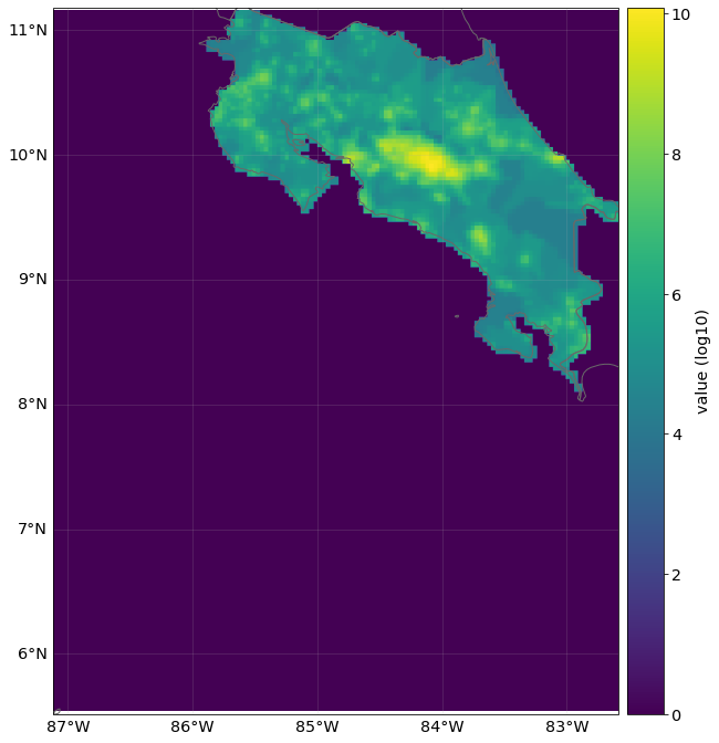
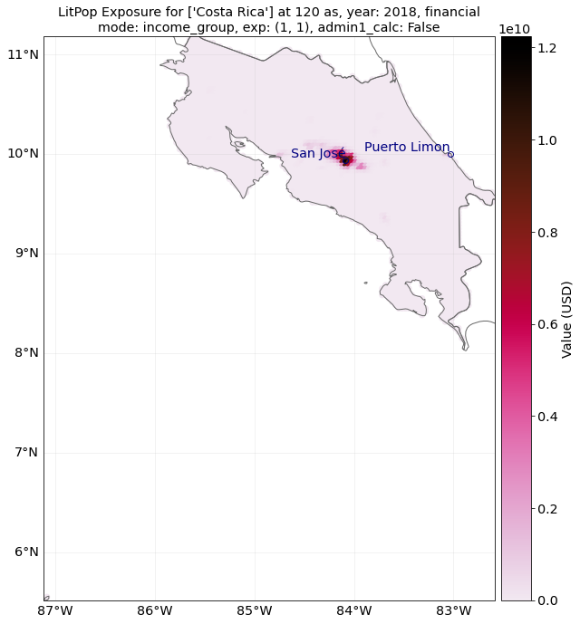
Let’s initiate an exposure instance with the financial mode “income_group” and at a resolution of 120 arcsec (roughly 4 km).
# Initiate a LitPop exposure entity for Costa Rica with varied resolution, fin_mode, and exponents:
exp = LitPop.from_countries(
    "Costa Rica", fin_mode="income_group", res_arcsec=120, exponents=(1, 1)
)  # change the parameters and see what happens...
# exp = LitPop.from_countries('Costa Rica', fin_mode='gdp', res_arcsec=90, exponents=(3,0)) # example of variation
exp.plot_raster()
# note the log scale of the colorbar
exp.plot_scatter();
2021-10-19 17:03:26,671 - climada.entity.exposures.litpop.gpw_population - WARNING - Reference year: 2018. Using nearest available year for GPW data: 2020
<GeoAxesSubplot:title={'center':"LitPop Exposure for ['Costa Rica'] at 120 as, year: 2018, financial\nmode: income_group, exp: (1, 1), admin1_calc: False"}>
Reference year#
Additionally, we can change the year our exposure is supposed to represent. For this, nightlight and population data are used that are closest to the requested years. Macroeconomic indicators like produced capital are interpolated from available data or scaled proportional to GDP.
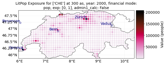
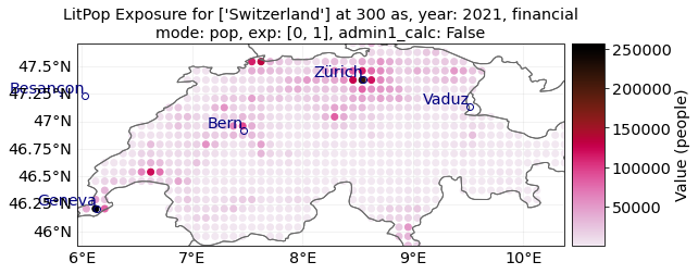
Let’s load a population exposure map for Switzerland in 2000 and 2021 with a resolution of 300 arcsec:
# You may want to check if you have downloaded dataset Gridded Population of the World (GPW), v4: Population Count, v4.11
# (2000 and 2020) first
pop_2000 = LitPop.from_countries(
    "CHE", fin_mode="pop", res_arcsec=300, exponents=(0, 1), reference_year=2000
)
# Alternatively, we ca use `from_population`:
pop_2021 = LitPop.from_population(
    countries="Switzerland", res_arcsec=300, reference_year=2021
)
# Since no population data for 2021 is available, the closest data point, 2020, is used (see LOGGER.warning)
pop_2000.plot_scatter()
pop_2021.plot_scatter()
"""Note the difference in total values on the color bar."""
2021-10-19 17:03:31,884 - climada.entity.exposures.litpop.gpw_population - WARNING - Reference year: 2021. Using nearest available year for GPW data: 2020
'Note the difference in total values on the color bar.'
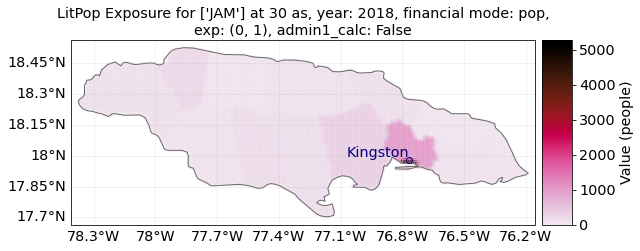
from_nightlight_intensity and from_population#
These wrapper methods can be used to produce exposures that are showing purely nightlight intensity or purely population count.
res = 30 # If you don't get an output after a very long time with country = "MEX", try with res = 100
country = "JAM" # Try different countries, i.e. 'JAM', 'CHE', 'RWA', 'MEX'
markersize = 4 # for plotting
buffer_deg = 0.04
exp_nightlights = LitPop.from_nightlight_intensity(
countries=country, res_arcsec=res
) # nightlight intensity
exp_nightlights.plot_hexbin(linewidth=markersize, buffer=buffer_deg)
# Compare to the population map:
exp_population = LitPop().from_population(countries=country, res_arcsec=res)
exp_population.plot_hexbin(linewidth=markersize, buffer=buffer_deg)
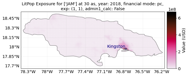
# Compare to default LitPop exposures:
exp = LitPop.from_countries(countries=country, res_arcsec=res)
exp.plot_hexbin(linewidth=markersize, buffer=buffer_deg);
2021-10-19 17:03:34,705 - climada.entity.exposures.litpop.gpw_population - WARNING - Reference year: 2018. Using nearest available year for GPW data: 2020
2021-10-19 17:03:35,308 - climada.entity.exposures.litpop.litpop - WARNING - Note: set_nightlight_intensity sets values to raw nightlight intensity, not to USD. To disaggregate asset value proportionally to nightlights^m, call from_countries or from_shape with exponents=(m,0).
2021-10-19 17:03:39,867 - climada.entity.exposures.litpop.gpw_population - WARNING - Reference year: 2018. Using nearest available year for GPW data: 2020
2021-10-19 17:03:44,032 - climada.entity.exposures.litpop.gpw_population - WARNING - Reference year: 2018. Using nearest available year for GPW data: 2020
<GeoAxesSubplot:title={'center':"LitPop Exposure for ['JAM'] at 30 as, year: 2018, financial mode: pc,\nexp: (1, 1), admin1_calc: False"}>
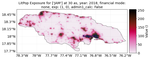
For Switzerland, population is resolved on the 3rd administrative level, with 2538 distinct geographical units. Therefore, the purely population-based map is highly resolved.
For Jamaica, population is only resolved on the 1st administrative level, with only 14 distinct geographical units. Therefore, the purely population-based map shows large monotonous patches. The combination of Lit and Pop results in a concentration of asset value estimates around the capital city Kingston.
Init LitPop-Exposure from custom shapes #
The methods LitPop.from_shape_and_countries and LitPop.from_shape initiate a LitPop-exposure instance for a given custom shape instead of a country. This can be used to initiate exposure for admin1-regions, i.e. cantons, states, districts, - but also for bounding boxes etc.
The difference between the two methods is that for from_shape_and_countries, the exposure for one or more whole countries is initiated first and then it is cropped to the shape. Please make sure that the shape is contained in the given countries.
With from_shape, the shape is initiated directly which is much more resource efficient but requires a total_value to be provided by the user.
A population exposure for a custom shape can be initiated directly via from_population without providing total_value.
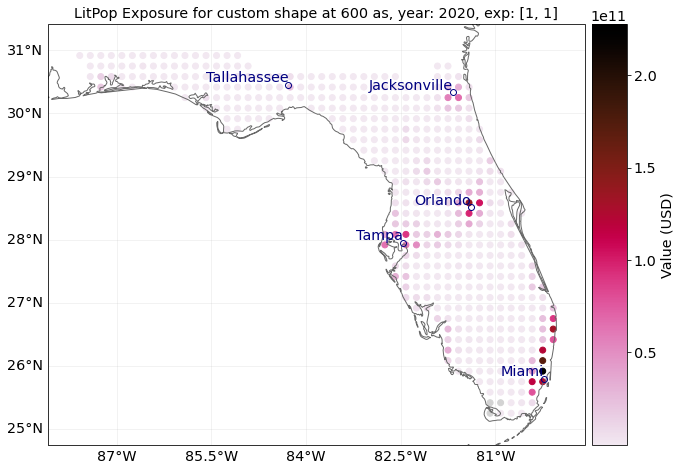
Example: State of Florida #
Using LitPop.from_shape_and_countries and LitPop.from_shape we initiate LitPop exposures for Florida:
import time
import climada.util.coordinates as u_coord
import climada.entity.exposures.litpop as lp

country_iso3a = "USA"
state_name = "Florida"
reslution_arcsec = 600
"""First, we need to get the shape of Florida:"""
admin1_info, admin1_shapes = u_coord.get_admin1_info(country_iso3a)
admin1_info = admin1_info[country_iso3a]
admin1_shapes = admin1_shapes[country_iso3a]
admin1_names = [record["name"] for record in admin1_info]
print(admin1_names)
for idx, name in enumerate(admin1_names):
    if admin1_names[idx] == state_name:
        break
print("Florida index: " + str(idx))

"""Secondly, we estimate the `total_value`"""
# `total_value` required user input for `from_shape`, here we assume 5% of total value of the whole USA:
total_value = 0.05 * lp._get_total_value_per_country(country_iso3a, "pc", 2020)

"""Then, we can initiate the exposures for Florida:"""
start = time.process_time()
exp = LitPop.from_shape(
    admin1_shapes[idx], total_value, res_arcsec=600, reference_year=2020
)
print(f"\n Runtime `from_shape` : {time.process_time() - start:1.2f} sec.\n")
exp.plot_scatter(vmin=100, buffer=0.5);
['Minnesota', 'Washington', 'Idaho', 'Montana', 'North Dakota', 'Michigan', 'Maine', 'Ohio', 'New Hampshire', 'New York', 'Vermont', 'Pennsylvania', 'Arizona', 'California', 'New Mexico', 'Texas', 'Alaska', 'Louisiana', 'Mississippi', 'Alabama', 'Florida', 'Georgia', 'South Carolina', 'North Carolina', 'Virginia', 'District of Columbia', 'Maryland', 'Delaware', 'New Jersey', 'Connecticut', 'Rhode Island', 'Massachusetts', 'Oregon', 'Hawaii', 'Utah', 'Wyoming', 'Nevada', 'Colorado', 'South Dakota', 'Nebraska', 'Kansas', 'Oklahoma', 'Iowa', 'Missouri', 'Wisconsin', 'Illinois', 'Kentucky', 'Arkansas', 'Tennessee', 'West Virginia', 'Indiana']
Florida index: 20
Runtime `from_shape` : 9.01 sec.
<GeoAxesSubplot:title={'center':'LitPop Exposure for custom shape at 600 as, year: 2020, exp: [1, 1]'}>
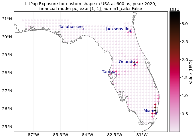
# `from_shape_and_countries` does not require `total_value`, but is slower to compute than `from_shape`,
# because first, the exposure for the whole USA is initiated:
start = time.process_time()
exp = LitPop.from_shape_and_countries(
    admin1_shapes[idx], country_iso3a, res_arcsec=600, reference_year=2020
)
print(
    f"\n Runtime `from_shape_and_countries` : {time.process_time() - start:1.2f} sec.\n"
)
exp.plot_scatter(vmin=100, buffer=0.5)
"""Note the differences in computational speed and total value between the two approaches"""
Runtime `from_shape_and_countries` : 24.49 sec.
'Note the differences in computational speed and total value between the two approaches'
Example: Zurich city area#
You can also define your own shape as a Polygon:
import time
from shapely.geometry import Polygon
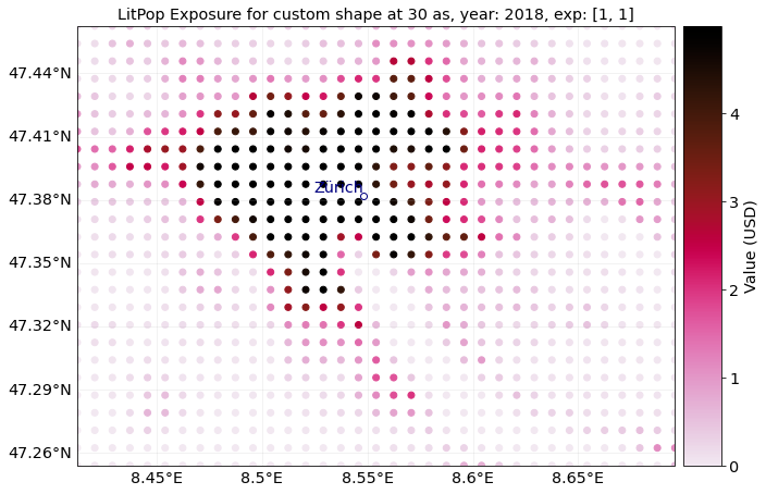
"""initiate LitPop exposures for a geographical box around the city of Zurich:"""
bounds = (8.41, 47.25, 8.70, 47.47) # (min_lon, max_lon, min_lat, max_lat)
total_value = 1000 # required user input for `from_shape`, here we just assume USD 1000 of total value
shape = Polygon(
[
(bounds[0], bounds[3]),
(bounds[2], bounds[3]),
(bounds[2], bounds[1]),
(bounds[0], bounds[1]),
]
)
import time
start = time.process_time()
exp = LitPop.from_shape(shape, total_value)
print(f"\n Runtime `from_shape` : {time.process_time() - start:1.2f} sec.\n")
exp.plot_scatter()
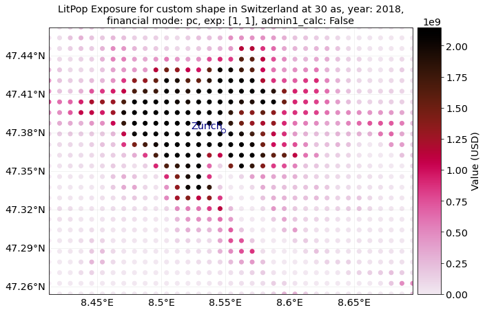
# `from_shape_and_countries` does not require `total_value`, but is slower to compute:
start = time.process_time()
exp = LitPop.from_shape_and_countries(shape, "Switzerland")
print(
f"\n Runtime `from_shape_and_countries` : {time.process_time() - start:1.2f} sec.\n"
)
exp.plot_scatter()
"""Note the difference in total value between the two exposure sets!"""
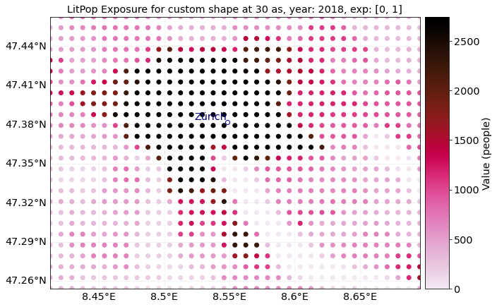
"""For comparison, initiate population exposure for a geographical box around the city of Zurich:"""
start = time.process_time()
exp_pop = LitPop.from_population(shape=shape)
print(f"\n Runtime `from_population` : {time.process_time() - start:1.2f} sec.\n")
exp_pop.plot_scatter()
"""Population exposure for a custom shape can be initiated directly via `set_population` without providing `total_value`"""
 Runtime `from_shape` : 0.51 sec.

2021-10-19 17:04:24,606 - climada.entity.exposures.litpop.gpw_population - WARNING - Reference year: 2018. Using nearest available year for GPW data: 2020

 Runtime `from_shape_and_countries` : 3.18 sec.
Runtime `from_population` : 0.75 sec.
'Population exposure for a custom shape can be initiated directly via `set_population` without providing `total_value`'
Sub-national (admin-1) GDP as intermediate downscaling layer #
In order to improve downscaling for countries with large regional differences within, a subnational breakdown of GDP can be used as an intermediate downscaling layer wherever available.
The sub-national (admin-1) GDP-breakdown needs to be added manually as a “.xls”-file to the folder data/system/GSDP in the CLIMADA-directory. Currently, such data is provided for more than 10 countries, including USA, India, and China.
The xls-file requires at least the following columns (with names specified in row 1):
State_Province: Names of admin-1 regions, i.e. states, cantons, provinces. Names need to match the naming of admin-1 shapes in the data used by the python packagecartopy.io(c.f.shapereader.natural_earth(name='admin_1_states_provinces'))GSDP_ref: value of sub-national GDP to be used (absolute or relative values)Postal, optional: Alternative identifier of region, if names do not match with cartopy. Needs to correspond to the Postal-identifiers used in the shapereader ofcartopy.io.
Please note that while admin1-GDP will per definition improve the downscaling of GDP, it might not necessarily improve the downscaling quality for other asset bases like produced capital (pc).
How To:#
The intermediate downscaling layer can be activated with the parameter admin1_calc=True.
# Initiate GDP-Entity for Switzerland, with and without admin1_calc:

ent_adm0 = LitPop.from_countries(
    "CHE", res_arcsec=120, fin_mode="gdp", admin1_calc=False
)
ent_adm0.check()

ent_adm1 = LitPop.from_countries(
    "CHE", res_arcsec=120, fin_mode="gdp", admin1_calc=True
)
ent_adm1.check()

print("Done.")
2021-10-19 17:04:31,363 - climada.entity.exposures.litpop.gpw_population - WARNING - Reference year: 2018. Using nearest available year for GPW data: 2020
Done.
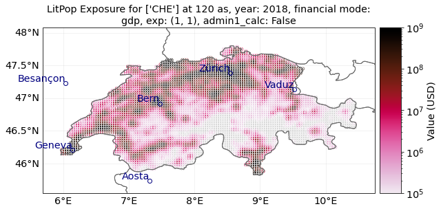
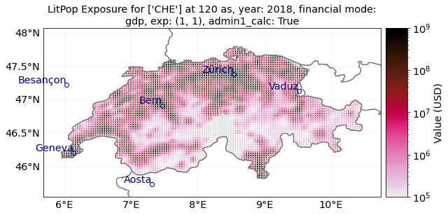
# Plotting:
from matplotlib import colors

norm = colors.LogNorm(vmin=1e5, vmax=1e9)  # setting range for the log-normal scale
markersize = 5
ent_adm0.plot_hexbin(buffer=0.3, norm=norm, linewidth=markersize)
ent_adm1.plot_hexbin(buffer=0.3, norm=norm, linewidth=markersize)

print("admin-0: First figure")
print("admin-1: Second figure")
"""Do you spot the small differences in Graubünden (eastern Switzerland)?"""
admin-0: First figure
admin-1: Second figure
'Do you spot the small differences in Graubünden (eastern Switzerland)?'