Hazard class

A Hazard contains the following information:

• tag (TagHazard): information about the source

• units (str): units of the intensity

• centroids (Centroids): centroids of the events

• event_id (np.array): id (>0) of each event

• event_name (list(str)): name of each event (default: event_id)

• date (np.array): integer date corresponding to the proleptic Gregorian ordinal, where January 1 of year 1 has ordinal 1 (ordinal format of datetime library)

• frequency (np.array): frequency of each event in seconds

• orig (np.array): flags indicating historical events (True) or probabilistic (False)

• intensity (sparse.csr_matrix): intensity of the events at centroids

• fraction (sparse.csr_matrix): fraction of affected exposures for each event at each centroid

Note that intensity and fraction are scipy.sparse matrices of size num_events x num_centroids. The Centroids class contains the geographical coordinates where the hazard is defined. A Centroids instance provides the coordinates either as points or raster data together with their Coordinate Reference System (CRS). The default CRS used in climada is the usual EPSG:4326. Centroids provides moreover methods to compute centroids areas, on land mask, country iso mask or distance to coast.

Read raster data

Raster data can be read in any format accepted by rasterio using Hazard’s set_raster() method. The raster information might refere to the intensity or fractionof the hazard. Different configuration options such as transforming the coordinates, changing the CRS and reading only a selected area or band are available through the set_raster() arguments as follows:

import numpy as np
from climada.hazard import Hazard
from climada.util.constants import HAZ_DEMO_FL

haz_ven = Hazard('FL')
# read intensity from raster file HAZ_DEMO_FL and set frequency for the contained event
haz_ven.set_raster([HAZ_DEMO_FL], attrs={'frequency':np.ones(1)/2})
haz_ven.check()

# per default the following attributes have been set
print('event_id: ', haz_ven.event_id)
print('event_name: ', haz_ven.event_name)
print('date: ', haz_ven.date)
print('frequency: ', haz_ven.frequency)
print('orig: ', haz_ven.orig)
print('min, max fraction: ', haz_ven.fraction.min(), haz_ven.fraction.max())

2019-06-18 20:16:31,574 - climada - DEBUG - Loading default config file: /Users/aznarsig/Documents/Python/climada_python/climada/conf/defaults.conf
2019-06-18 20:16:33,143 - climada.util.coordinates - INFO - Reading /Users/aznarsig/Documents/Python/climada_python/data/demo/SC22000_VE__M1.grd.gz
event_id:  [1]
event_name:  ['1']
date:  [1.]
frequency:  [0.5]
orig:  [ True]
min, max fraction:  0.0 1.0

EXERCISE:

1. Read raster data in EPSG 2201 Coordinate Reference System (CRS)

2. Read raster data in its given CRS and transform it to the affine transformation Affine(0.009000000000000341, 0.0, -69.33714959699981, 0.0, -0.009000000000000341, 10.42822096697894), height=500, width=501)

3. Read raster data in window Window(10, 10, 20, 30)

# Put your code here

# Solution:

# 1. The CRS can be reprojected using dst_crs option
haz = Hazard('FL')
haz.set_raster([HAZ_DEMO_FL], dst_crs={'init':'epsg:2201'})
haz.check()
print('Solution 1:')
print('centroids CRS:', haz.centroids.crs)
print('raster info:', haz.centroids.meta)

# 2. Transformations of the coordinates can be set using the transform option and Affine
from rasterio import Affine
haz = Hazard('FL')
haz.set_raster([HAZ_DEMO_FL], transform=Affine(0.009000000000000341, 0.0, -69.33714959699981, \
                                               0.0, -0.009000000000000341, 10.42822096697894), height=500, width=501)
haz.check()
print('Solution 2:')
print('raster info:', haz.centroids.meta)
print('intensity size:', haz.intensity.shape)

# 3. A partial part of the raster can be loaded using the window or geometry
from rasterio.windows import Window
haz = Hazard('FL')
haz.set_raster([HAZ_DEMO_FL], window=Window(10, 10, 20, 30))
haz.check()
print('raster info:', haz.centroids.meta)
print('intensity size:', haz.intensity.shape)

2019-06-18 20:16:35,529 - climada.util.coordinates - INFO - Reading /Users/aznarsig/Documents/Python/climada_python/data/demo/SC22000_VE__M1.grd.gz
Solution 1:
centroids CRS: {'init': 'epsg:2201'}
raster info: {'driver': 'GSBG', 'dtype': 'float32', 'nodata': 1.701410009187828e+38, 'width': 978, 'height': 1091, 'count': 1, 'crs': {'init': 'epsg:2201'}, 'transform': Affine(1011.5372910988809, 0.0, 1120744.548666424,
       0.0, -1011.5372910988809, 1189133.7652687668)}
2019-06-18 20:16:37,942 - climada.util.coordinates - INFO - Reading /Users/aznarsig/Documents/Python/climada_python/data/demo/SC22000_VE__M1.grd.gz
Solution 2:
raster info: {'driver': 'GSBG', 'dtype': 'float32', 'nodata': 1.701410009187828e+38, 'width': 501, 'height': 500, 'count': 1, 'crs': CRS.from_dict(init='epsg:4326'), 'transform': Affine(0.009000000000000341, 0.0, -69.33714959699981,
       0.0, -0.009000000000000341, 10.42822096697894)}
intensity size: (1, 250500)
2019-06-18 20:16:40,244 - climada.util.coordinates - INFO - Reading /Users/aznarsig/Documents/Python/climada_python/data/demo/SC22000_VE__M1.grd.gz
raster info: {'driver': 'GSBG', 'dtype': 'float32', 'nodata': 1.701410009187828e+38, 'width': 20, 'height': 30, 'count': 1, 'crs': CRS.from_dict(init='epsg:4326'), 'transform': Affine(0.009000000000000341, 0.0, -69.2471495969998,
       0.0, -0.009000000000000341, 10.338220966978936)}
intensity size: (1, 600)

Fast visualization of raster data with plot_raster():

# The masked values of the raster are set to 0
# Sometimes the raster file does not contain all the information, as in this case the mask value -9999
# We mask it manuall and plot it using plot_raster()
haz_ven.intensity[haz_ven.intensity==-9999] = 0
haz_ven.plot_raster()

<matplotlib.image.AxesImage at 0x1c2e835fd0>

haz_ven.plot_intensity(1) # takes longer. plots with resolution RESOLUTION of climada.util.plot

/Users/aznarsig/anaconda3/envs/climada_up/lib/python3.7/site-packages/matplotlib/tight_layout.py:176: UserWarning: Tight layout not applied. The left and right margins cannot be made large enough to accommodate all axes decorations.
  warnings.warn('Tight layout not applied. The left and right margins '

(<Figure size 648x936 with 2 Axes>,
 array([[<cartopy.mpl.geoaxes.GeoAxesSubplot object at 0x1c2cf23ef0>]],
       dtype=object))

Read other formats

• excel: Hazards can be read from Excel files following the template in climada_python/data/system/hazard_template.xlsx using the read_excel() method.

• MATLAB: Hazards generated with CLIMADA’s MATLAB version (.mat format) can be read using read_mat().

• vector data: Use Hazard’s set_vector() to read shape data (all formats supported by fiona.

• hdf5: Hazards generated with the CLIMADA in Python (.h5 format) can be read using read_hdf5().

from climada.hazard import Hazard
from climada.util import HAZ_DEMO_H5 # CLIMADA's Python file
# Hazard needs to know the acronym of the hazard type to be constructed!!! Use 'NA' if not known.
haz_tc_fl = Hazard('TC')
haz_tc_fl.read_hdf5(HAZ_DEMO_H5)  # Historic and synthetic tropical cyclones in Florida from 1975 to 2011
haz_tc_fl.check() # Use always the check() method to see if the hazard has been loaded correctly

2019-06-18 20:17:03,625 - climada.hazard.base - INFO - Reading /Users/aznarsig/Documents/Python/climada_python/data/demo/tc_fl_1975_2011.h5

/Users/aznarsig/anaconda3/envs/climada_up/lib/python3.7/site-packages/h5py/_hl/dataset.py:313: H5pyDeprecationWarning: dataset.value has been deprecated. Use dataset[()] instead.
  "Use dataset[()] instead.", H5pyDeprecationWarning)

 Define a Hazard by hand

A Hazard can be defined by filling its values one by one, as follows:

# setting points
import numpy as np
from scipy import sparse

lat = np.array([26.933899, 26.957203, 26.783846, 26.645524, 26.897796, 26.925359, \
       26.914768, 26.853491, 26.845099, 26.82651 , 26.842772, 26.825905, \
       26.80465 , 26.788649, 26.704277, 26.71005 , 26.755412, 26.678449, \
       26.725649, 26.720599, 26.71255 , 26.6649  , 26.664699, 26.663149, \
       26.66875 , 26.638517, 26.59309 , 26.617449, 26.620079, 26.596795, \
       26.577049, 26.524585, 26.524158, 26.523737, 26.520284, 26.547349, \
       26.463399, 26.45905 , 26.45558 , 26.453699, 26.449999, 26.397299, \
       26.4084  , 26.40875 , 26.379113, 26.3809  , 26.349068, 26.346349, \
       26.348015, 26.347957])

lon = np.array([-80.128799, -80.098284, -80.748947, -80.550704, -80.596929, \
       -80.220966, -80.07466 , -80.190281, -80.083904, -80.213493, \
       -80.0591  , -80.630096, -80.075301, -80.069885, -80.656841, \
       -80.190085, -80.08955 , -80.041179, -80.1324  , -80.091746, \
       -80.068579, -80.090698, -80.1254  , -80.151401, -80.058749, \
       -80.283371, -80.206901, -80.090649, -80.055001, -80.128711, \
       -80.076435, -80.080105, -80.06398 , -80.178973, -80.110519, \
       -80.057701, -80.064251, -80.07875 , -80.139247, -80.104316, \
       -80.188545, -80.21902 , -80.092391, -80.1575  , -80.102028, \
       -80.16885 , -80.116401, -80.08385 , -80.241305, -80.158855])

n_cen = lon.size # number of centroids
n_ev = 10 # number of events

haz = Hazard('TC')
haz.centroids.set_lat_lon(lat, lon) # default crs used
haz.intensity = sparse.csr_matrix(np.random.random((n_ev, n_cen)))
haz.units = 'm'
haz.event_id = np.arange(n_ev, dtype=int)
haz.event_name = ['ev_12', 'ev_21', 'Maria', 'ev_35', 'Irma', 'ev_16', 'ev_15', 'Edgar', 'ev_1', 'ev_9']
haz.date = [721166, 734447, 734447, 734447, 721167, 721166, 721167, 721200, 721166, 721166]
haz.orig = np.zeros(n_ev, bool)
haz.frequency = np.ones(n_ev)/n_ev
haz.fraction = haz.intensity.copy()
haz.fraction.data.fill(1)
haz.check()
haz.centroids.plot()

(<Figure size 648x936 with 1 Axes>,
 <cartopy.mpl.geoaxes.GeoAxesSubplot at 0x1c2e8f34a8>)

# setting raster
import numpy as np
from scipy import sparse

# raster info:
# border upper left corner (of the pixel, not of the center of the pixel)
xf_lat = 22
xo_lon = -72
# resolution in lat and lon
d_lat = -0.5 # negative because starting in upper corner
d_lon = 0.5 # same step as d_lat
# number of points
n_lat = 50
n_lon = 40

n_ev = 10 # number of events

haz = Hazard('TC')
haz.centroids.set_raster_from_pix_bounds(xf_lat, xo_lon, d_lat, d_lon, n_lat, n_lon) # default crs used
haz.intensity = sparse.csr_matrix(np.random.random((n_ev, haz.centroids.size)))
haz.units = 'm'
haz.event_id = np.arange(n_ev, dtype=int)
haz.event_name = ['ev_12', 'ev_21', 'Maria', 'ev_35', 'Irma', 'ev_16', 'ev_15', 'Edgar', 'ev_1', 'ev_9']
haz.date = [721166, 734447, 734447, 734447, 721167, 721166, 721167, 721200, 721166, 721166]
haz.orig = np.zeros(n_ev, bool)
haz.frequency = np.ones(n_ev)/n_ev
haz.fraction = haz.intensity.copy()
haz.fraction.data.fill(1)
haz.check()
print('Check centroids borders:', haz.centroids.total_bounds)
haz.centroids.plot()

# using set_raster_from_pnt_bounds, the bounds refer to the bounds of the center of the pixel
left, bottom, right, top = xo_lon, -3.0, -52.0, xf_lat
haz.centroids.set_raster_from_pnt_bounds((left, bottom, right, top), 0.5) # default crs used
print('Check centroids borders:', haz.centroids.total_bounds)

Check centroids borders: (-72.0, -3.0, -52.0, 22.0)
Check centroids borders: (-72.25, -3.25, -51.75, 22.25)

Methods

The following methods can be used to analyse the data in Hazard:

• calc_year_set() method returns a dictionary with all the historical (not synthetic) event ids that happened at each year.

• get_event_date() returns strings of dates in ISO format.

• To obtain the relation between event ids and event names, two methods can be used get_event_name() and get_event_id().

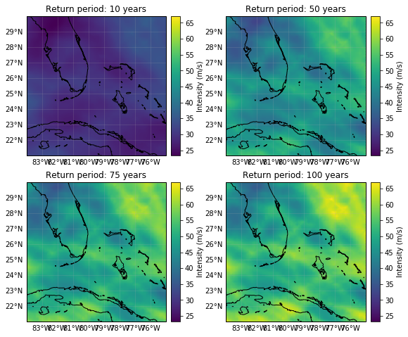
Other methods to handle one or several Hazards are: - the property size returns the number of events contained. - append() is used to expand events with data from another Hazard (and sam centroids). - select() returns a new hazard with the selected region, date and/or synthetic or historical filter. - remove_duplicates(): removes events with same name and date. - local_exceedance_inten() returns a matrix with the exceedence frequency at every frequency and provided return periods. This is the one used in plot_rp_intensity().

Centroids methods: - centroids properties such as area per pixel, distance to coast, country iso or on land mask are available through differen set_XX()methods. - set_lat_lon_to_meta() computes the raster meta dictionary from present lat and lon. set_meta_to_lat_lon() computes lat and lon of the center of the pixels described in attribute meta. The raster meta information contains at least: width, height, crs and transform data (use help(Centroids) for more info). Using raster centroids can increase computing performance for several computations. - when using lats and lons (vector data) the geopandas.GeoSeries geometry attribute contains the CRS information and can be filled with point shapes to perform different computation. The geometry points can be then released using empty_geometry_points().

EXERCISE:

Using the previous hazard haz_tc_fl answer these questions: 1. How many synthetic events are contained? 2. Generate an hazard with historical hurricanes ocurring between 1995 and 2001. 3. How many historical hurricanes occured in 1999? Which was the year with most hurricanes between 1995 and 2001? 4. What is the number of centroids with distance to coast smaller than 1km?

# Put your code here:

#help(hist_tc.centroids)

# SOLUTION:

# 1.How many synthetic events are contained?
print('Number of total events:', haz_tc_fl.size)
print('Number of synthetic events:', np.logical_not(haz_tc_fl.orig).astype(int).sum())

# 2. Generate a hazard with historical hurricanes ocurring between 1995 and 2001.
hist_tc = haz_tc_fl.select(date=('1995-01-01', '2001-12-31'), orig=True)
print('Number of historical events between 1995 and 2001:', hist_tc.size)

# 3. How many historical hurricanes occured in 1999? Which was the year with most hurricanes between 1995 and 2001?
ev_per_year = hist_tc.calc_year_set() # events ids per year
print('Number of events in 1999:', ev_per_year[1999].size)
max_year = 1995
max_ev = ev_per_year[1995].size
for year, ev in ev_per_year.items():
    if ev.size > max_ev:
        max_year = year
print('Year with most hurricanes between 1995 and 2001:', max_year)

# 4. What is the number of centroids with distance to coast smaller than 1km?
hist_tc.centroids.set_dist_coast()
num_cen_coast = np.argwhere(hist_tc.centroids.dist_coast < 1000).size
print('Number of centroids close to coast: ', num_cen_coast)

Number of total events: 2405
Number of synthetic events: 1924
Number of historical events between 1995 and 2001: 109
Number of events in 1999: 16
Year with most hurricanes between 1995 and 2001: 1995
Number of centroids close to coast:  28

 Visualize Hazards

There are three different plot functions: plot_intensity(), plot_fraction()and plot_rp_intensity(). Depending on the inputs, different properties can be visualized. Check the documentation of the functions:

help(haz_tc_fl.plot_intensity)
help(haz_tc_fl.plot_rp_intensity)

Help on method plot_intensity in module climada.hazard.base:

plot_intensity(event=None, centr=None, **kwargs) method of climada.hazard.base.Hazard instance
    Plot intensity values for a selected event or centroid.

    Parameters:
        event (int or str, optional): If event > 0, plot intensities of
            event with id = event. If event = 0, plot maximum intensity in
            each centroid. If event < 0, plot abs(event)-largest event. If
            event is string, plot events with that name.
        centr (int or tuple, optional): If centr > 0, plot intensity
            of all events at centroid with id = centr. If centr = 0,
            plot maximum intensity of each event. If centr < 0,
            plot abs(centr)-largest centroid where higher intensities
            are reached. If tuple with (lat, lon) plot intensity of nearest
            centroid.
        kwargs (optional): arguments for pcolormesh matplotlib function
            used in event plots

    Returns:
        matplotlib.figure.Figure, matplotlib.axes._subplots.AxesSubplot

    Raises:
        ValueError

Help on method plot_rp_intensity in module climada.hazard.base:

plot_rp_intensity(return_periods=(25, 50, 100, 250), **kwargs) method of climada.hazard.base.Hazard instance
    Compute and plot hazard exceedance intensity maps for different
    return periods. Calls local_exceedance_inten.

    Parameters:
        return_periods (tuple(int), optional): return periods to consider
        kwargs (optional): arguments for pcolormesh matplotlib function
            used in event plots

    Returns:
        matplotlib.figure.Figure, matplotlib.axes._subplots.AxesSubplot,
        np.ndarray (return_periods.size x num_centroids)

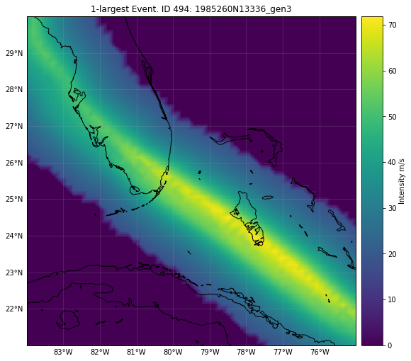
# 1. intensities of the largest event (defined as greater sum of intensities):
# all events:
haz_tc_fl.plot_intensity(event=-1) # 1985260N13336_gen3 is a synthetic event
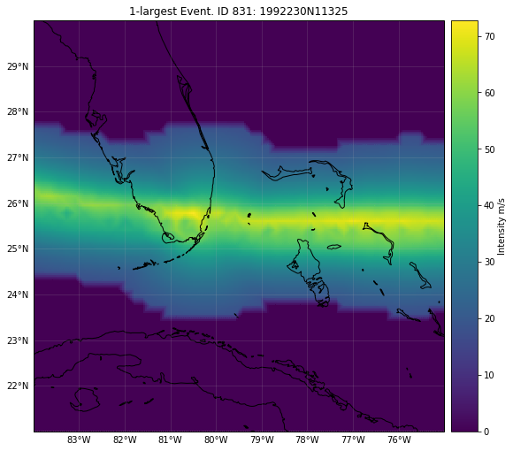
# only historical events:
haz_tc_fl.select(orig=True).plot_intensity(-1) # largest historical event: 1992230N11325 hurricane ANDREW

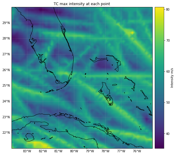
# 2. maximum intensities at each centroid:
haz_tc_fl.plot_intensity(event=0)

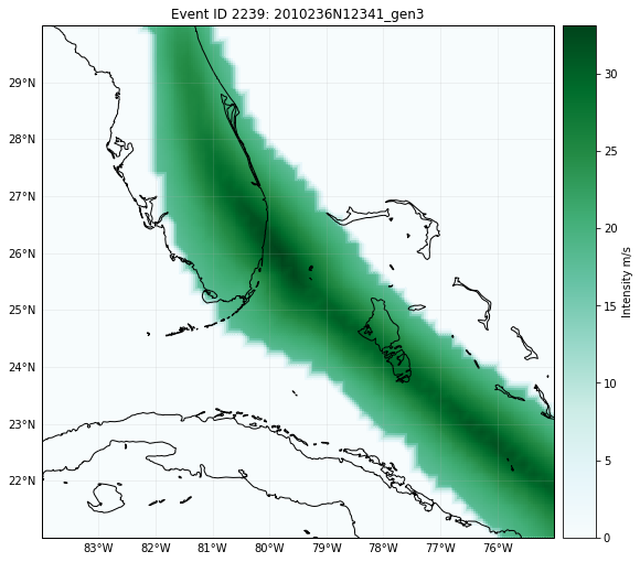
# 3. intensities of hurricane 2010236N12341_gen3:
haz_tc_fl.plot_intensity(event='2010236N12341_gen3', cmap='BuGn') # setting color map

# 4. tropical cyclone intensities maps for the return periods [10, 50, 75, 100]
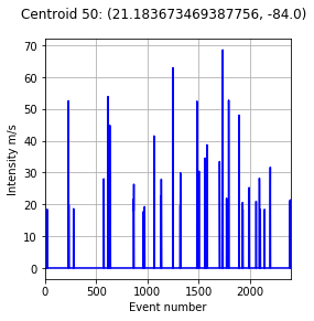
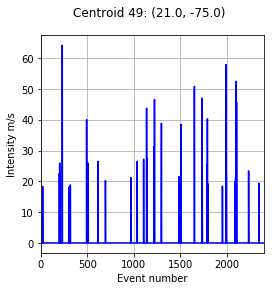
_, _, res = haz_tc_fl.plot_rp_intensity([10, 50, 75, 100])

# 5. intensities of all the events in centroid with id 50
haz_tc_fl.plot_intensity(centr=50)

# 5. intensities of all the events in centroid closest to lat, lon = (26.5, -81)
haz_tc_fl.plot_intensity(centr=(26.5, -81));

/Users/aznarsig/anaconda3/envs/climada_up/lib/python3.7/site-packages/matplotlib/tight_layout.py:176: UserWarning: Tight layout not applied. The left and right margins cannot be made large enough to accommodate all axes decorations.
  warnings.warn('Tight layout not applied. The left and right margins '

2019-06-18 20:17:08,112 - climada.hazard.base - INFO - Computing exceedance intenstiy map for return periods: [ 10  50  75 100]

/Users/aznarsig/anaconda3/envs/climada_up/lib/python3.7/site-packages/matplotlib/tight_layout.py:176: UserWarning: Tight layout not applied. The left and right margins cannot be made large enough to accommodate all axes decorations.
  warnings.warn('Tight layout not applied. The left and right margins '

2019-06-18 20:17:10,137 - climada.hazard.centroids.centr - INFO - Setting geometry points.

 Write a hazard

Hazards can be written and read in hdf5 format as follows:

haz_tc_fl.write_hdf5('results/haz_tc_fl.h5')

haz = Hazard('TC')
haz.read_hdf5('results/haz_tc_fl.h5')
haz.check()

2019-06-18 20:17:17,555 - climada.hazard.base - INFO - Writting results/haz_tc_fl.h5
2019-06-18 20:17:18,752 - climada.hazard.base - INFO - Reading results/haz_tc_fl.h5

/Users/aznarsig/anaconda3/envs/climada_up/lib/python3.7/site-packages/h5py/_hl/dataset.py:313: H5pyDeprecationWarning: dataset.value has been deprecated. Use dataset[()] instead.
  "Use dataset[()] instead.", H5pyDeprecationWarning)

GeoTiff data is generated using write_raster():

haz_ven.write_raster('results/haz_ven.tif') # each event is a band of the tif file

2019-06-18 20:17:18,786 - climada.util.coordinates - INFO - Writting results/haz_ven.tif

Pickle will work as well:

from climada.util.save import save
# this generates a results folder in the current path and stores the output there
save('tutorial_haz_tc_fl.p', haz_tc_fl)

2019-06-18 20:17:18,835 - climada.util.save - INFO - Written file /Users/aznarsig/Documents/Python/tutorial/results/tutorial_haz_tc_fl.p