Exposures class
Exposure can describe the geographical distribution of people, livelihoods and assets or infrastructure; all items potentially exposed to hazards. It is represented in the class Exposures, which is a GeoDataFrame of Python’s library geopandas.
The variables (columns) and metada contained are:
tag (Tag): metada - information about the source data
ref_year (int): metada - reference year
value_unit (str): metada - unit of the exposures values
latitude (pd.Series): latitude
longitude (pd.Series): longitude
value (pd.Series): a value for each exposure
if_ (pd.Series, optional): e.g. if_TC. impact functions ids for hazard TC. There might be different hazards defined: if_TC, if_FL, … If not provided, set to default
if_with ids 1 in check().geometry (pd.Series, optional): geometry of type Point of each instance. Computed in method
set_geometry_points()meta (dict): dictionary containing corresponding raster properties (if any): width, height, crs and transform must be present at least (transform needs to contain upper left corner!). Exposures might not contain all the points of the corresponding raster.
deductible (pd.Series, optional): deductible value for each exposure. Used for insurance
cover (pd.Series, optional): cover value for each exposure. Used for insurance
category_id (pd.Series, optional): category id (e.g. building code) for each exposure
region_id (pd.Series, optional): region id (e.g. country ISO code) for each exposure
centr_* (pd.Series, optional): e.g. centr_TC. centroids index for hazard TC. There might be different hazards defined: centr_TC, centr_FL, … Computed in method
assign_centroids()
Some of the variables are optional. This means that the package climada.engine also works without these variables set. For instance, the region_id and category_id values only provide additional information, whilst the centr_* variable can be computed if not provided using the method assign_centroids(). The attibute geometry is only needed to execute the methods of geopandas and can be set using the method set_geometry_points().
if_ is the most important attribute, since it relates the exposures to the hazard by specifying the impact functions. Ideally it should be set to the specific hazard (e.g. if_TC) so that different hazards can be set in the same Exposures (e.g. if_TC and if_FL). If there isn’t any if_* value provided, the check() method puts a default if_ with ones which can be used by the impact calculation in engine.
After defining an Exposures instance use always the check() method to see which attributes are missing. This method will raise an ERROR if value, longitude or latitude ar missing and an INFO messages for the the optional variables not set.
Define Exposures from a DataFrame
[1]:
import numpy as np
from pandas import DataFrame
from climada.entity import Exposures

# Fill DataFrame
exp_df = DataFrame()
n_exp = 100*100
exp_df['value'] = np.arange(n_exp) # provide value
lat, lon = np.mgrid[15 : 35 : complex(0, np.sqrt(n_exp)), 20 : 40 : complex(0, np.sqrt(n_exp))]
exp_df['latitude'] = lat.flatten() # provide latitude
exp_df['longitude'] = lon.flatten() # provide longitude
exp_df['if_TC'] = np.ones(n_exp, int) # provide impact functions for TC or any other peril

print('\x1b[1;03;30;30m' + 'exp_df is a DataFrame:', str(type(exp_df)) + '\x1b[0m')
print('\x1b[1;03;30;30m' + 'exp_df looks like:' + '\x1b[0m')
print(exp_df.head())

# Generate Exposures
exp_df = Exposures(exp_df)
print('\n' + '\x1b[1;03;30;30m' + 'exp_df is now an Exposures:', str(type(exp_df)) + '\x1b[0m')
exp_df.set_geometry_points() # set geometry attribute (shapely Points) from GeoDataFrame from latitude and longitude
print('\n' + '\x1b[1;03;30;30m' + 'check method logs:' + '\x1b[0m')
exp_df.check() # puts metadata that has not been assigned

print('\n' + '\x1b[1;03;30;30m'  + 'exp_df looks like:' + '\x1b[0m')
print(exp_df.head())
2020-03-13 16:27:06,555 - climada - DEBUG - Loading default config file: /Users/aznarsig/Documents/Python/climada_python/climada/conf/defaults.conf
exp_df is a DataFrame: <class 'pandas.core.frame.DataFrame'>
exp_df looks like:
   value  latitude  longitude  if_TC
0      0      15.0  20.000000      1
1      1      15.0  20.202020      1
2      2      15.0  20.404040      1
3      3      15.0  20.606061      1
4      4      15.0  20.808081      1

exp_df is now an Exposures: <class 'climada.entity.exposures.base.Exposures'>
2020-03-13 16:27:08,988 - climada.util.coordinates - INFO - Setting geometry points.

check method logs:
2020-03-13 16:27:09,546 - climada.entity.exposures.base - INFO - crs set to default value: {'init': 'epsg:4326', 'no_defs': True}
2020-03-13 16:27:09,547 - climada.entity.exposures.base - INFO - tag metadata set to default value:  File:
 Description:
2020-03-13 16:27:09,548 - climada.entity.exposures.base - INFO - ref_year metadata set to default value: 2018
2020-03-13 16:27:09,548 - climada.entity.exposures.base - INFO - value_unit metadata set to default value: USD
2020-03-13 16:27:09,550 - climada.entity.exposures.base - INFO - meta metadata set to default value: None
2020-03-13 16:27:09,551 - climada.entity.exposures.base - INFO - centr_ not set.
2020-03-13 16:27:09,552 - climada.entity.exposures.base - INFO - deductible not set.
2020-03-13 16:27:09,553 - climada.entity.exposures.base - INFO - cover not set.
2020-03-13 16:27:09,553 - climada.entity.exposures.base - INFO - category_id not set.
2020-03-13 16:27:09,555 - climada.entity.exposures.base - INFO - region_id not set.

exp_df looks like:
   value  latitude  longitude  if_TC                      geometry
0      0      15.0  20.000000      1                 POINT (20 15)
1      1      15.0  20.202020      1   POINT (20.2020202020202 15)
2      2      15.0  20.404040      1   POINT (20.4040404040404 15)
3      3      15.0  20.606061      1  POINT (20.60606060606061 15)
4      4      15.0  20.808081      1  POINT (20.80808080808081 15)
Define Exposures from a GeoDataFrame with POINT geometry
[2]:
import numpy as np
import geopandas as gpd
from climada.entity import Exposures

# Fill GeoDataFrame
world = gpd.read_file(gpd.datasets.get_path('naturalearth_cities'))
print('\x1b[1;03;30;30m' + 'World is a GeoDataFrame:', str(type(world)) + '\x1b[0m')
print('\x1b[1;03;30;30m' + 'World looks like:' + '\x1b[0m')
print(world.head())

# Generate Exposures
exp_gpd = Exposures(world)
print('\n' + '\x1b[1;03;30;30m' + 'exp_gpd is now an Exposures:', str(type(exp_gpd)) + '\x1b[0m')
exp_gpd['value'] = np.arange(world.shape[0]) # provide value
exp_gpd.set_lat_lon() # set latitude and longitude attributes from geometry
exp_gpd['if_TC'] = np.ones(world.shape[0], int) # provide impact functions for TC or any other peril

print('\n' + '\x1b[1;03;30;30m' + 'check method logs:' + '\x1b[0m')
exp_gpd.check() # puts metadata that has not been assigned

print('\n' + '\x1b[1;03;30;30m'  + 'exp_gpd looks like:' + '\x1b[0m')
print(exp_gpd.head())
World is a GeoDataFrame: <class 'geopandas.geodataframe.GeoDataFrame'>
World looks like:
           name                                     geometry
0  Vatican City  POINT (12.45338654497177 41.90328217996012)
1    San Marino    POINT (12.44177015780014 43.936095834768)
2         Vaduz  POINT (9.516669472907267 47.13372377429357)
3    Luxembourg  POINT (6.130002806227083 49.61166037912108)
4       Palikir  POINT (158.1499743237623 6.916643696007725)

exp_gpd is now an Exposures: <class 'climada.entity.exposures.base.Exposures'>
2020-03-13 16:27:09,599 - climada.entity.exposures.base - INFO - Setting latitude and longitude attributes.

check method logs:
2020-03-13 16:27:09,612 - climada.entity.exposures.base - INFO - crs set to default value: {'init': 'epsg:4326', 'no_defs': True}
2020-03-13 16:27:09,613 - climada.entity.exposures.base - INFO - tag metadata set to default value:  File:
 Description:
2020-03-13 16:27:09,614 - climada.entity.exposures.base - INFO - ref_year metadata set to default value: 2018
2020-03-13 16:27:09,616 - climada.entity.exposures.base - INFO - value_unit metadata set to default value: USD
2020-03-13 16:27:09,617 - climada.entity.exposures.base - INFO - meta metadata set to default value: None
2020-03-13 16:27:09,618 - climada.entity.exposures.base - INFO - centr_ not set.
2020-03-13 16:27:09,620 - climada.entity.exposures.base - INFO - deductible not set.
2020-03-13 16:27:09,621 - climada.entity.exposures.base - INFO - cover not set.
2020-03-13 16:27:09,623 - climada.entity.exposures.base - INFO - category_id not set.
2020-03-13 16:27:09,624 - climada.entity.exposures.base - INFO - region_id not set.

exp_gpd looks like:
           name                                     geometry  value  \
0  Vatican City  POINT (12.45338654497177 41.90328217996012)      0
1    San Marino    POINT (12.44177015780014 43.936095834768)      1
2         Vaduz  POINT (9.516669472907267 47.13372377429357)      2
3    Luxembourg  POINT (6.130002806227083 49.61166037912108)      3
4       Palikir  POINT (158.1499743237623 6.916643696007725)      4

    latitude   longitude  if_TC
0  41.903282   12.453387      1
1  43.936096   12.441770      1
2  47.133724    9.516669      1
3  49.611660    6.130003      1
4   6.916644  158.149974      1
Read Exposures of an excel file
Excel files can be ingested directly following the template provided in climada_python/data/system/entity_template.xlsx, in the sheet assets.
[3]:
# An excel file with the variables defined in the template can be directly ingested using these commands
import pandas as pd
from climada.util.constants import ENT_TEMPLATE_XLS
from climada.entity import Exposures

# Fill DataFrame from Excel file
file_name = ENT_TEMPLATE_XLS # provide absolute path of the excel file
exp_templ = pd.read_excel(file_name)

print('\x1b[1;03;30;30m' + 'exp_templ is a DataFrame:', str(type(exp_templ)) + '\x1b[0m')
print('\x1b[1;03;30;30m' + 'exp_templ looks like:' + '\x1b[0m')
print(exp_templ.head())

# Generate Exposures
exp_templ = Exposures(exp_templ)
print('\n' + '\x1b[1;03;30;30m' + 'exp_templ is now an Exposures:', str(type(exp_templ)) + '\x1b[0m')
exp_templ.set_geometry_points() # set geometry attribute (shapely Points) from GeoDataFrame from latitude and longitude
print('\n' + '\x1b[1;03;30;30m' + 'check method logs:' + '\x1b[0m')
exp_templ.check() # puts metadata that has not been assigned

print('\n' + '\x1b[1;03;30;30m'  + 'exp_templ looks like:' + '\x1b[0m')
print(exp_templ.head())
exp_templ is a DataFrame: <class 'pandas.core.frame.DataFrame'>
exp_templ looks like:
    latitude  longitude         value  deductible         cover  region_id  \
0  26.933899 -80.128799  1.392750e+10           0  1.392750e+10          1
1  26.957203 -80.098284  1.259606e+10           0  1.259606e+10          1
2  26.783846 -80.748947  1.259606e+10           0  1.259606e+10          1
3  26.645524 -80.550704  1.259606e+10           0  1.259606e+10          1
4  26.897796 -80.596929  1.259606e+10           0  1.259606e+10          1

   category_id  if_TC  centr_TC  if_FL  centr_FL
0            1      1         1      1         1
1            1      1         2      1         2
2            1      1         3      1         3
3            1      1         4      1         4
4            1      1         5      1         5

exp_templ is now an Exposures: <class 'climada.entity.exposures.base.Exposures'>
2020-03-13 16:27:09,737 - climada.util.coordinates - INFO - Setting geometry points.

check method logs:
2020-03-13 16:27:09,740 - climada.entity.exposures.base - INFO - crs set to default value: {'init': 'epsg:4326', 'no_defs': True}
2020-03-13 16:27:09,741 - climada.entity.exposures.base - INFO - tag metadata set to default value:  File:
 Description:
2020-03-13 16:27:09,742 - climada.entity.exposures.base - INFO - ref_year metadata set to default value: 2018
2020-03-13 16:27:09,743 - climada.entity.exposures.base - INFO - value_unit metadata set to default value: USD
2020-03-13 16:27:09,744 - climada.entity.exposures.base - INFO - meta metadata set to default value: None

exp_templ looks like:
    latitude  longitude         value  deductible         cover  region_id  \
0  26.933899 -80.128799  1.392750e+10           0  1.392750e+10          1
1  26.957203 -80.098284  1.259606e+10           0  1.259606e+10          1
2  26.783846 -80.748947  1.259606e+10           0  1.259606e+10          1
3  26.645524 -80.550704  1.259606e+10           0  1.259606e+10          1
4  26.897796 -80.596929  1.259606e+10           0  1.259606e+10          1

   category_id  if_TC  centr_TC  if_FL  centr_FL  \
0            1      1         1      1         1
1            1      1         2      1         2
2            1      1         3      1         3
3            1      1         4      1         4
4            1      1         5      1         5

                               geometry
0          POINT (-80.128799 26.933899)
1  POINT (-80.09828400000001 26.957203)
2          POINT (-80.748947 26.783846)
3          POINT (-80.550704 26.645524)
4          POINT (-80.596929 26.897796)
Read Exposures of any file type supported by GeoDataFrame and DataFrame
Geopandas can read almost any vector-based spatial data format including ESRI shapefile, GeoJSON files and more, see readers geopandas. Pandas supports formats such as csv, html or sql; see readers pandas. Using the corresponding readers, DataFrame and GeoDataFrame can be filled and provided to Exposures following the previous examples.
Read Exposures from a raster file
Raster data contained in files of any format supported by rasterio can be charged using set_from_raster(). The attribute meta containing the raster properties is then set.
[4]:
# dummy example
from rasterio.windows import Window
from climada.util.constants import HAZ_DEMO_FL
exp = Exposures()
exp.set_from_raster(HAZ_DEMO_FL, window= Window(10, 20, 50, 60)) # check all the options (e.g. change CRS)
exp.check()
print('Meta:', exp.meta)
2020-03-13 16:27:09,766 - climada.util.coordinates - INFO - Reading /Users/aznarsig/Documents/Python/climada_python/data/demo/SC22000_VE__M1.grd.gz
2020-03-13 16:27:09,815 - climada.entity.exposures.base - INFO - ref_year metadata set to default value: 2018
2020-03-13 16:27:09,816 - climada.entity.exposures.base - INFO - value_unit metadata set to default value: USD
2020-03-13 16:27:09,817 - climada.entity.exposures.base - INFO - Setting if_ to default impact functions ids 1.
2020-03-13 16:27:09,818 - climada.entity.exposures.base - INFO - centr_ not set.
2020-03-13 16:27:09,819 - climada.entity.exposures.base - INFO - deductible not set.
2020-03-13 16:27:09,820 - climada.entity.exposures.base - INFO - cover not set.
2020-03-13 16:27:09,821 - climada.entity.exposures.base - INFO - category_id not set.
2020-03-13 16:27:09,823 - climada.entity.exposures.base - INFO - region_id not set.
2020-03-13 16:27:09,824 - climada.entity.exposures.base - INFO - geometry not set.
Meta: {'driver': 'GSBG', 'dtype': 'float32', 'nodata': 1.701410009187828e+38, 'width': 50, 'height': 60, 'count': 1, 'crs': CRS.from_dict(init='epsg:4326'), 'transform': Affine(0.009000000000000341, 0.0, -69.2471495969998,
       0.0, -0.009000000000000341, 10.248220966978932)}
Read exposures generated by CLIMADA
The methods read_mat() will read Exposures generated by CLIMADA’s MATLAB version and read_hdf5() will read the ones generated CLIMADA in Python. These methods will allow to read all the metadata in addition to the GeoDataFrame.
Methods
[5]:
# read MATLAB file from climada MATLAB version with read_mat()
# and the ones generated with the Python version with read_hdf5()
from climada.util.constants import EXP_DEMO_H5

exp_hdf5 = Exposures()
exp_hdf5.read_hdf5(EXP_DEMO_H5)
exp_hdf5.check()
print(type(exp_hdf5))
2020-03-13 16:27:09,835 - climada.entity.exposures.base - INFO - Reading /Users/aznarsig/Documents/Python/climada_python/data/demo/exp_demo_today.h5
2020-03-13 16:27:09,947 - climada.entity.exposures.base - INFO - meta metadata set to default value: None
2020-03-13 16:27:09,948 - climada.entity.exposures.base - INFO - centr_ not set.
<class 'climada.entity.exposures.base.Exposures'>
[6]:
# add sea points
from climada.entity import add_sea
exp_templ_sea = add_sea(exp_templ, (10, 5)) # 10km from coast and at 5km resolution
exp_templ_sea.check()
exp_templ_sea.tail() # region_id set to -1 for the sea points
2020-03-13 16:27:09,957 - climada.entity.exposures.base - INFO - Adding sea at 5 km resolution and 10 km distance from coast.
2020-03-13 16:27:10,390 - climada.util.coordinates - INFO - Setting geometry points.
[6]:
| latitude | longitude | value | deductible | cover | region_id | category_id | if_TC | centr_TC | if_FL | centr_FL | geometry | |
|---|---|---|---|---|---|---|---|---|---|---|---|---|
| 58 | 27.005495 | -79.939012 | 0.0 | 0 | 0.0 | -1 | 0 | 0 | 0 | 0 | 0 | POINT (-79.93901179481654 27.00549520230383) |
| 59 | 27.050492 | -80.074001 | 0.0 | 0 | 0.0 | -1 | 0 | 0 | 0 | 0 | 0 | POINT (-80.07400099568045 27.05049160259181) |
| 60 | 27.050492 | -80.029005 | 0.0 | 0 | 0.0 | -1 | 0 | 0 | 0 | 0 | 0 | POINT (-80.02900459539248 27.05049160259181) |
| 61 | 27.050492 | -79.984008 | 0.0 | 0 | 0.0 | -1 | 0 | 0 | 0 | 0 | 0 | POINT (-79.98400819510451 27.05049160259181) |
| 62 | 27.050492 | -79.939012 | 0.0 | 0 | 0.0 | -1 | 0 | 0 | 0 | 0 | 0 | POINT (-79.93901179481654 27.05049160259181) |
all the methods from GeoDataFrame
Have a look into all the possible methods provided by GeoDataFrame. They will allow you to perform operations like the following:
[7]:
# extract data in a region: latitudes between -5 and 5
sel_exp = exp_gpd.cx[:, -5:5]
sel_exp # the output is of type GeoDataFrame
[7]:
| name | geometry | value | latitude | longitude | if_TC | |
|---|---|---|---|---|---|---|
| 9 | Tarawa | POINT (173.0175708285494 1.338187505624603) | 9 | 1.338188 | 173.017571 | 1 |
| 13 | Kigali | POINT (30.05858591906411 -1.95164421006325) | 13 | -1.951644 | 30.058586 | 1 |
| 15 | Juba | POINT (31.58002559278731 4.829975198277964) | 15 | 4.829975 | 31.580026 | 1 |
| 27 | Bujumbura | POINT (29.3600060615284 -3.376087220374643) | 27 | -3.376087 | 29.360006 | 1 |
| 48 | Kampala | POINT (32.58137766712105 0.318604813383331) | 48 | 0.318605 | 32.581378 | 1 |
| 65 | Mogadishu | POINT (45.36473175245874 2.068627192947531) | 65 | 2.068627 | 45.364732 | 1 |
| 79 | Quito | POINT (-78.5019969671124 -0.2130423220355624) | 79 | -0.213042 | -78.501997 | 1 |
| 84 | Malabo | POINT (8.783277545821136 3.750015278026183) | 84 | 3.750015 | 8.783278 | 1 |
| 90 | Libreville | POINT (9.457965045823698 0.3853886097185182) | 90 | 0.385389 | 9.457965 | 1 |
| 98 | Brazzaville | POINT (15.28274363384867 -4.257239913197509) | 98 | -4.257240 | 15.282744 | 1 |
| 103 | Bandar Seri Begawan | POINT (114.9332840566623 4.883331114619239) | 103 | 4.883331 | 114.933284 | 1 |
| 106 | Bangui | POINT (18.55828812528728 4.366644306349087) | 106 | 4.366644 | 18.558288 | 1 |
| 107 | Yaounde | POINT (11.51470489685443 3.868646520754112) | 107 | 3.868647 | 11.514705 | 1 |
| 124 | Victoria | POINT (55.44998978559113 -4.6166316539734) | 124 | -4.616632 | 55.449990 | 1 |
| 125 | Sao Tome | POINT (6.733325153234773 0.3334021188329075) | 125 | 0.333402 | 6.733325 | 1 |
| 128 | Male | POINT (73.499947467955 4.1667081898118) | 128 | 4.166708 | 73.499947 | 1 |
| 147 | Kuala Lumpur | POINT (101.6980374167464 3.168611730712371) | 147 | 3.168612 | 101.698037 | 1 |
| 176 | Kinshasa | POINT (15.31302602317174 -4.327778243275986) | 176 | -4.327778 | 15.313026 | 1 |
| 194 | Nairobi | POINT (36.81471100047145 -1.281400883237779) | 194 | -1.281401 | 36.814711 | 1 |
| 196 | Bogota | POINT (-74.08528981377441 4.598369421147822) | 196 | 4.598369 | -74.085290 | 1 |
| 201 | Singapore | POINT (103.853874819099 1.294979325105942) | 201 | 1.294979 | 103.853875 | 1 |
[8]:
# extract data in a polygon
from shapely.geometry import Polygon

poly = Polygon([(0, -10), (0, 10), (10, 5)])
sel_exp = exp_gpd[exp_gpd.intersects(poly)]
sel_exp # the output is of type Exposures
[8]:
| name | geometry | value | latitude | longitude | if_TC | |
|---|---|---|---|---|---|---|
| 36 | Lome | POINT (1.22081126074562 6.133882930268385) | 36 | 6.133883 | 1.220811 | 1 |
| 84 | Malabo | POINT (8.783277545821136 3.750015278026183) | 84 | 3.750015 | 8.783278 | 1 |
| 113 | Cotonou | POINT (2.518044740568598 6.401954422782467) | 113 | 6.401954 | 2.518045 | 1 |
| 125 | Sao Tome | POINT (6.733325153234773 0.3334021188329075) | 125 | 0.333402 | 6.733325 | 1 |
[9]:
# change reference system
sel_exp.to_crs(epsg=3395, inplace=True) # use help to see more options: help(sel_exp.to_crs)
sel_exp.crs
[9]:
{'init': 'epsg:3395', 'no_defs': True}
[10]:
# concatenate exposures
import pandas as pd

exp_all = pd.concat([exp_templ, exp_df], ignore_index=True, sort=False)

# the output is of type Exposures
print('exp_all type and number of rows:', type(exp_all), exp_all.shape[0])

# NaNs will appear in the missing values
exp_all.tail()
exp_all type and number of rows: <class 'climada.entity.exposures.base.Exposures'> 10024
[10]:
| latitude | longitude | value | deductible | cover | region_id | category_id | if_TC | centr_TC | if_FL | centr_FL | geometry | |
|---|---|---|---|---|---|---|---|---|---|---|---|---|
| 10019 | 35.0 | 39.191919 | 9995.0 | NaN | NaN | NaN | NaN | 1 | NaN | NaN | NaN | POINT (39.19191919191919 35) |
| 10020 | 35.0 | 39.393939 | 9996.0 | NaN | NaN | NaN | NaN | 1 | NaN | NaN | NaN | POINT (39.39393939393939 35) |
| 10021 | 35.0 | 39.595960 | 9997.0 | NaN | NaN | NaN | NaN | 1 | NaN | NaN | NaN | POINT (39.5959595959596 35) |
| 10022 | 35.0 | 39.797980 | 9998.0 | NaN | NaN | NaN | NaN | 1 | NaN | NaN | NaN | POINT (39.7979797979798 35) |
| 10023 | 35.0 | 40.000000 | 9999.0 | NaN | NaN | NaN | NaN | 1 | NaN | NaN | NaN | POINT (40 35) |
[11]:
# remove values
exp_all_1 = exp_all.drop([1]) # delete row 1
print('\x1b[1;03;30;30m' + 'Row 1 deleted:' + '\x1b[0m')
print(exp_all_1.head())
exp_all_val = exp_all.drop(['value'], axis=1) # delete colomn 'value'
print('\x1b[1;03;30;30m' + 'Column value deleted:' + '\x1b[0m')
print(exp_all_val.head())
Row 1 deleted:
    latitude  longitude         value  deductible         cover  region_id  \
0  26.933899 -80.128799  1.392750e+10         0.0  1.392750e+10        1.0
2  26.783846 -80.748947  1.259606e+10         0.0  1.259606e+10        1.0
3  26.645524 -80.550704  1.259606e+10         0.0  1.259606e+10        1.0
4  26.897796 -80.596929  1.259606e+10         0.0  1.259606e+10        1.0
5  26.925359 -80.220966  1.259606e+10         0.0  1.259606e+10        1.0

   category_id  if_TC  centr_TC  if_FL  centr_FL                      geometry
0          1.0      1       1.0    1.0       1.0  POINT (-80.128799 26.933899)
2          1.0      1       3.0    1.0       3.0  POINT (-80.748947 26.783846)
3          1.0      1       4.0    1.0       4.0  POINT (-80.550704 26.645524)
4          1.0      1       5.0    1.0       5.0  POINT (-80.596929 26.897796)
5          1.0      1       6.0    1.0       6.0  POINT (-80.220966 26.925359)
Column value deleted:
    latitude  longitude  deductible         cover  region_id  category_id  \
0  26.933899 -80.128799         0.0  1.392750e+10        1.0          1.0
1  26.957203 -80.098284         0.0  1.259606e+10        1.0          1.0
2  26.783846 -80.748947         0.0  1.259606e+10        1.0          1.0
3  26.645524 -80.550704         0.0  1.259606e+10        1.0          1.0
4  26.897796 -80.596929         0.0  1.259606e+10        1.0          1.0

   if_TC  centr_TC  if_FL  centr_FL                              geometry
0      1       1.0    1.0       1.0          POINT (-80.128799 26.933899)
1      1       2.0    1.0       2.0  POINT (-80.09828400000001 26.957203)
2      1       3.0    1.0       3.0          POINT (-80.748947 26.783846)
3      1       4.0    1.0       4.0          POINT (-80.550704 26.645524)
4      1       5.0    1.0       5.0          POINT (-80.596929 26.897796)
Visualize Exposures
The method plot_hexbin() uses cartopy and matplotlib’s hexbin function to represent the exposures values as 2d bins over a map. Configure your plot by fixing the different inputs of the method or by modifying the returned matplotlib figure and axes.
[12]:
# execute 'Define Exposures from a DataFrame' to see the results
print('\x1b[1;03;30;30m' + 'Plotting exp_df.' + '\x1b[0m')
axs = exp_df.plot_hexbin()
axs.set_xlim(15, 45) # modify x-axis borders
axs.set_ylim(10, 40) # modify y-axis borders

# use buffer option to enlarge borders of plot
# use gridsize to change bins size
exp_df.plot_hexbin(pop_name=False, buffer=1.0, gridsize=200)
Plotting exp_df.
/Users/aznarsig/Documents/Python/climada_python/climada/util/plot.py:311: UserWarning: Tight layout not applied. The left and right margins cannot be made large enough to accommodate all axes decorations.
  fig.tight_layout()
[12]:
<cartopy.mpl.geoaxes.GeoAxesSubplot at 0x1c2a328198>
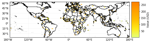
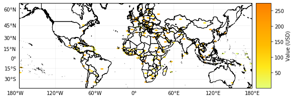
[13]:
# execute 'Define Exposures from a GeoDataFrame with POINT geometry' to see the results
print('\x1b[1;03;30;30m' + 'Plotting exp_gpd.' + '\x1b[0m')
exp_gpd.plot_hexbin(pop_name=False)

# when the geometry is changed, the plot is adapted correspondingly
exp_gpd.to_crs({'init':'epsg:3395'}, inplace=True)
exp_gpd.plot_hexbin(pop_name=False)
Plotting exp_gpd.
2020-03-13 16:27:17,828 - climada.entity.exposures.base - INFO - Setting latitude and longitude attributes.
[13]:
<cartopy.mpl.geoaxes.GeoAxesSubplot at 0x1c2a4e7a90>
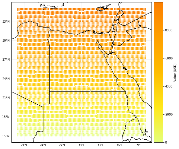
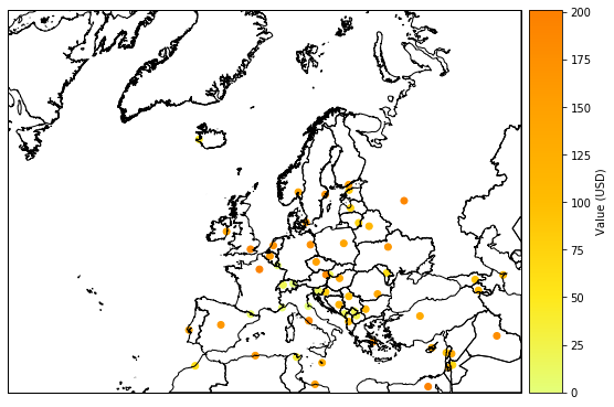
The method plot_scatter() uses cartopy and matplotlib’s scatter function to represent the points values over a 2d map. As usal, it returns the figure and axes, which can be modify aftwerwards.
[14]:
exp_gpd.to_crs({'init':'epsg:3035'}, inplace=True)
exp_gpd.plot_scatter(pop_name=False)
2020-03-13 16:27:31,559 - climada.entity.exposures.base - INFO - Setting latitude and longitude attributes.
[14]:
<cartopy.mpl.geoaxes.GeoAxesSubplot at 0x1c29b3c978>
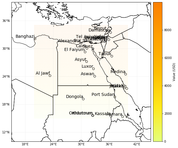
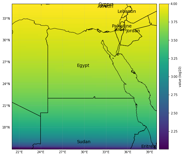
The method plot_raster() rasterizes the points into the given resolution. Use the save_tiff option to save the resulting tiff file.
[15]:
from climada.util.plot import add_cntry_names # use climada's plotting utilities
ax = exp_df.plot_raster() # plot with same resolution as data
add_cntry_names(ax, [exp_df.longitude.min(), exp_df.longitude.max(), exp_df.latitude.min(), exp_df.latitude.max()])
# use plot_raster(save_tiff) to save the corresponding raster in tiff format
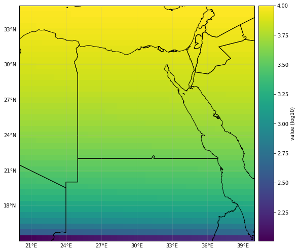
# change raster resolution
ax = exp_df.plot_raster(raster_res=0.5, save_tiff='results/exp_df.tiff')
2020-03-13 16:27:37,088 - climada.util.coordinates - INFO - Raster from resolution 0.20202020202019355 to 0.20202020202019355.
2020-03-13 16:27:39,086 - climada.util.coordinates - INFO - Raster from resolution 0.20202020202019355 to 0.5.
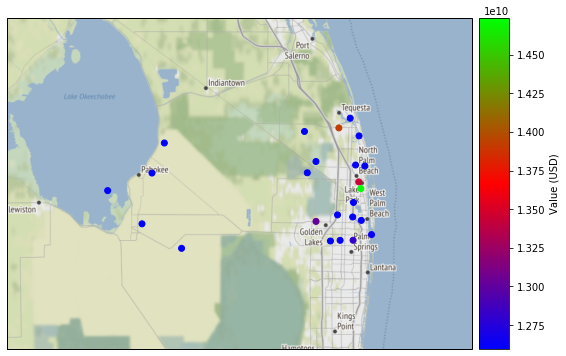
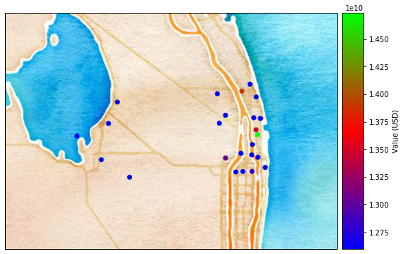
Finally, the method plot_basemap() plots the scatter points over a satellite image using contextily library:
[16]:
import contextily as ctx
# select the background image from the available ctx.sources
ax = exp_templ.plot_basemap(buffer=30000, cmap='brg') # using open street map
ax = exp_templ.plot_basemap(buffer=30000, url=ctx.sources.ST_WATERCOLOR, cmap='brg', zoom=9) # set image zoom
2020-03-13 16:27:41,624 - climada.entity.exposures.base - INFO - Setting latitude and longitude attributes.
/Users/aznarsig/anaconda3/envs/climada_env/lib/python3.7/site-packages/contextily/tile.py:199: FutureWarning: The url format using 'tileX', 'tileY', 'tileZ' as placeholders is deprecated. Please use '{x}', '{y}', '{z}' instead.
  FutureWarning,
2020-03-13 16:27:43,082 - climada.entity.exposures.base - INFO - Setting latitude and longitude attributes.
2020-03-13 16:27:43,089 - climada.entity.exposures.base - INFO - Setting latitude and longitude attributes.
2020-03-13 16:27:44,200 - climada.entity.exposures.base - INFO - Setting latitude and longitude attributes.
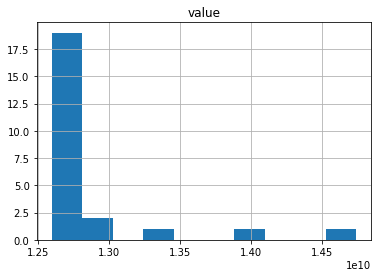
Since Exposures is a GeoDataFrame, any function for visualization from geopandas can be used. Check making maps and examples gallery.
[17]:
# other visualization types
exp_templ.hist(column='value')
[17]:
array([[<matplotlib.axes._subplots.AxesSubplot object at 0x1c2eb21128>]],
      dtype=object)
Write Exposures
Exposures can be saved in any format available for GeoDataFrame (see fiona.supported_drivers) and DataFrame (pandas IO tools). Take into account that in many of these formats the metadata (e.g. variables ref_year, value_unit and tag) will not be saved. Use instead the format hdf5 provided by Exposures methods write_hdf5() and read_hdf5() to handle all the data.
[18]:
# GeoDataFrame formats
import fiona; fiona.supported_drivers

# GeoDataFrame default: ESRI shape file in current path. metadata not saved!
exp_templ.to_file('results/exp_templ')

# DataFrame save to csv format. geometry writen as string, metadata not saved!
exp_templ.to_csv('results/exp_templ_csv', sep='\t')
[19]:
# write
exp_templ.write_hdf5('results/exp_temp.h5')
# read
exp_read = Exposures()
exp_read.read_hdf5('results/exp_temp.h5')
exp_read.head()
2020-03-13 16:27:44,859 - climada.entity.exposures.base - INFO - Writting results/exp_temp.h5
2020-03-13 16:27:44,881 - climada.entity.exposures.base - INFO - Reading results/exp_temp.h5
/Users/aznarsig/anaconda3/envs/climada_env/lib/python3.7/site-packages/IPython/core/interactiveshell.py:3331: PerformanceWarning:
your performance may suffer as PyTables will pickle object types that it cannot
map directly to c-types [inferred_type->mixed,key->block2_values] [items->['geometry']]

  exec(code_obj, self.user_global_ns, self.user_ns)
[19]:
| latitude | longitude | value | deductible | cover | region_id | category_id | if_TC | centr_TC | if_FL | centr_FL | geometry | |
|---|---|---|---|---|---|---|---|---|---|---|---|---|
| 0 | 26.933899 | -80.128799 | 1.392750e+10 | 0 | 1.392750e+10 | 1 | 1 | 1 | 1 | 1 | 1 | POINT (-80.12879899999999 26.93389899999996) |
| 1 | 26.957203 | -80.098284 | 1.259606e+10 | 0 | 1.259606e+10 | 1 | 1 | 1 | 2 | 1 | 2 | POINT (-80.09828400000001 26.957203) |
| 2 | 26.783846 | -80.748947 | 1.259606e+10 | 0 | 1.259606e+10 | 1 | 1 | 1 | 3 | 1 | 3 | POINT (-80.748947 26.783846) |
| 3 | 26.645524 | -80.550704 | 1.259606e+10 | 0 | 1.259606e+10 | 1 | 1 | 1 | 4 | 1 | 4 | POINT (-80.550704 26.645524) |
| 4 | 26.897796 | -80.596929 | 1.259606e+10 | 0 | 1.259606e+10 | 1 | 1 | 1 | 5 | 1 | 5 | POINT (-80.596929 26.89779599999996) |
Finallly, as with any Python object, use climada’s save option to save it in pickle format.
[20]:
# save in pickle format
from climada.util.save import save
# this generates a results folder in the current path and stores the output there
save('exp_templ.pkl.p', exp_templ) # creates results folder and stores there
2020-03-13 16:27:44,911 - climada.util.save - INFO - Written file /Users/aznarsig/Documents/Python/climada_python/doc/tutorial/results/exp_templ.pkl.p
Dask - improving performance for big exposure
Dask is used in some methods of CLIMADA and can be activated easily by proving the scheduler.
[21]:
# set_geometry_points is expensive for big exposures
# for small amount of data, the execution time might be even greater when using dask
exp_df.drop(columns=['geometry'], inplace=True)
print(exp_df.head())
exp_df.set_geometry_points(scheduler='processes')
print(exp_df.head())
   value  latitude  longitude  if_TC
0      0      15.0  20.000000      1
1      1      15.0  20.202020      1
2      2      15.0  20.404040      1
3      3      15.0  20.606061      1
4      4      15.0  20.808081      1
2020-03-13 16:27:44,921 - climada.util.coordinates - INFO - Setting geometry points.
   value  latitude  longitude  if_TC                      geometry
0      0      15.0  20.000000      1                 POINT (20 15)
1      1      15.0  20.202020      1   POINT (20.2020202020202 15)
2      2      15.0  20.404040      1   POINT (20.4040404040404 15)
3      3      15.0  20.606061      1  POINT (20.60606060606061 15)
4      4      15.0  20.808081      1  POINT (20.80808080808081 15)