SupplyChain class
[1]:
import numpy as np
import pandas as pd
from climada.hazard import TCTracks, TropCyclone, Centroids
from climada.entity import LitPop
from climada.entity import ImpactFuncSet, IFTropCyclone
from climada.engine import SupplyChain
C:\Users\aleciu\Anaconda3\envs\climada_env\lib\site-packages\pandas_datareader\compat\__init__.py:7: FutureWarning: pandas.util.testing is deprecated. Use the functions in the public API at pandas.testing instead.
  from pandas.util.testing import assert_frame_equal
This tutorial shows how to use the SupplyChain class of CLIMADA. This class allows assessing indirect impacts via Input-Ouput modeling. Before diving into this class, it is highly recommended the user first familiarizes herself with the Exposures, Hazard and Impact classes.
1. Load Multi-Regional Input-Output Tables (MRIOT) data.
At first, one needs to load Input Output data. SupplyChain has a function to download and read multi-regional input-output tables (MRIOT) from the 2016 release of WIOD project (www.wiod.org). Yearly WIOT tables are available for the period 2000-2014. A table is automatically downloaded the first time it is used.
[2]:
supplychain = SupplyChain()
supplychain.read_wiod16(year=2012)
2021-03-30 15:07:55,814 - climada.util.files_handler - INFO - Downloading http://www.wiod.org/protected3/data16/wiot_ROW/WIOT2012_Nov16_ROW.xlsb to file C:\Users\aleciu\climada\data\WIOD\WIOT2012_Nov16_ROW.xlsb
60.6kKB [00:10, 5.78kKB/s]
2021-03-30 15:08:06,307 - climada.engine.supplychain - INFO - Downloading WIOD table for year 2012
Let’s now look at what data are now loaded into SupplyChain, i.e. modelled countries, sectors and IO data structure.
[3]:
supplychain.mriot_reg_names
[3]:
array(['AUS', 'AUT', 'BEL', 'BGR', 'BRA', 'CAN', 'CHE', 'CHN', 'CYP',
       'CZE', 'DEU', 'DNK', 'ESP', 'EST', 'FIN', 'FRA', 'GBR', 'GRC',
       'HRV', 'HUN', 'IDN', 'IND', 'IRL', 'ITA', 'JPN', 'KOR', 'LTU',
       'LUX', 'LVA', 'MEX', 'MLT', 'NLD', 'NOR', 'POL', 'PRT', 'ROU',
       'RUS', 'SVK', 'SVN', 'SWE', 'TUR', 'TWN', 'USA', 'ROW'],
      dtype=object)
There are 43 countries plus 1. The additional “country” refers to all countries not explicitly modeled which are aggregated into a Rest of World (ROW) “country”.
[4]:
supplychain.sectors
[4]:
array(['Crop and animal production, hunting and related service activities',
       'Forestry and logging', 'Fishing and aquaculture',
       'Mining and quarrying',
       'Manufacture of food products, beverages and tobacco products',
       'Manufacture of textiles, wearing apparel and leather products',
       'Manufacture of wood and of products of wood and cork, except furniture; manufacture of articles of straw and plaiting materials',
       'Manufacture of paper and paper products',
       'Printing and reproduction of recorded media',
       'Manufacture of coke and refined petroleum products ',
       'Manufacture of chemicals and chemical products ',
       'Manufacture of basic pharmaceutical products and pharmaceutical preparations',
       'Manufacture of rubber and plastic products',
       'Manufacture of other non-metallic mineral products',
       'Manufacture of basic metals',
       'Manufacture of fabricated metal products, except machinery and equipment',
       'Manufacture of computer, electronic and optical products',
       'Manufacture of electrical equipment',
       'Manufacture of machinery and equipment n.e.c.',
       'Manufacture of motor vehicles, trailers and semi-trailers',
       'Manufacture of other transport equipment',
       'Manufacture of furniture; other manufacturing',
       'Repair and installation of machinery and equipment',
       'Electricity, gas, steam and air conditioning supply',
       'Water collection, treatment and supply',
       'Sewerage; waste collection, treatment and disposal activities; materials recovery; remediation activities and other waste management services ',
       'Construction',
       'Wholesale and retail trade and repair of motor vehicles and motorcycles',
       'Wholesale trade, except of motor vehicles and motorcycles',
       'Retail trade, except of motor vehicles and motorcycles',
       'Land transport and transport via pipelines', 'Water transport',
       'Air transport',
       'Warehousing and support activities for transportation',
       'Postal and courier activities',
       'Accommodation and food service activities',
       'Publishing activities',
       'Motion picture, video and television programme production, sound recording and music publishing activities; programming and broadcasting activities',
       'Telecommunications',
       'Computer programming, consultancy and related activities; information service activities',
       'Financial service activities, except insurance and pension funding',
       'Insurance, reinsurance and pension funding, except compulsory social security',
       'Activities auxiliary to financial services and insurance activities',
       'Real estate activities',
       'Legal and accounting activities; activities of head offices; management consultancy activities',
       'Architectural and engineering activities; technical testing and analysis',
       'Scientific research and development',
       'Advertising and market research',
       'Other professional, scientific and technical activities; veterinary activities',
       'Administrative and support service activities',
       'Public administration and defence; compulsory social security',
       'Education', 'Human health and social work activities',
       'Other service activities',
       'Activities of households as employers; undifferentiated goods- and services-producing activities of households for own use',
       'Activities of extraterritorial organizations and bodies'],
      dtype=object)
[5]:
print(supplychain.sectors.shape)
(56,)
There are 56 economic sectors. These sectors can also be grouped into higher-level sectors. For instance, in the aftermath we will model the service sector which will include the following sectors:
[6]:
supplychain.sectors[range(26,56)]
[6]:
array(['Construction',
       'Wholesale and retail trade and repair of motor vehicles and motorcycles',
       'Wholesale trade, except of motor vehicles and motorcycles',
       'Retail trade, except of motor vehicles and motorcycles',
       'Land transport and transport via pipelines', 'Water transport',
       'Air transport',
       'Warehousing and support activities for transportation',
       'Postal and courier activities',
       'Accommodation and food service activities',
       'Publishing activities',
       'Motion picture, video and television programme production, sound recording and music publishing activities; programming and broadcasting activities',
       'Telecommunications',
       'Computer programming, consultancy and related activities; information service activities',
       'Financial service activities, except insurance and pension funding',
       'Insurance, reinsurance and pension funding, except compulsory social security',
       'Activities auxiliary to financial services and insurance activities',
       'Real estate activities',
       'Legal and accounting activities; activities of head offices; management consultancy activities',
       'Architectural and engineering activities; technical testing and analysis',
       'Scientific research and development',
       'Advertising and market research',
       'Other professional, scientific and technical activities; veterinary activities',
       'Administrative and support service activities',
       'Public administration and defence; compulsory social security',
       'Education', 'Human health and social work activities',
       'Other service activities',
       'Activities of households as employers; undifferentiated goods- and services-producing activities of households for own use',
       'Activities of extraterritorial organizations and bodies'],
      dtype=object)
Weather to aggregate sectors into main sectors and how to do it is up to the user, according to the application of interest and data availability. Default settings are available in CLIMADA based on the built-in datasets. These will be introduced below when calculating direct damages.
[7]:
supplychain.mriot_data
[7]:
array([[11105.733356382272, 315.7113177373571, 179.43254266338693, ...,
        9.093853356314124, 0, 1.1873518978687656e-06],
       [116.88308162207898, 139.3046230501366, 0.4165797269551787, ...,
        0.016109951596559337, 0, 2.9150840971500206e-08],
       [22.556627754337466, 0.011392711240065655, 23.191690635397794,
        ..., 0.02463511351049634, 0, 2.9671358991110717e-09],
       ...,
       [2.0888621906340483, 0.06898124909560921, 0.18736619171021462,
        ..., 15914.85428702459, 0, 0.7881946937807305],
       [0.041425098917944464, 4.0179492086967524e-05,
        0.00019545212518185459, ..., 0, 0, 0],
       [0, 0, 0, ..., 0, 0, 0]], dtype=object)
[8]:
supplychain.mriot_data.shape
[8]:
(2464, 2464)
The MRIO table is a squared matrix with columns (and rows) equal to the number of economic sectors times the number of modeled countries, i.e. 56x44 = 2464. Each column (row) reports input (output) data of all sectors of a given country untill all countries are reported. The total production from all subsectors of all countries is:
[9]:
supplychain.total_prod
[9]:
array([71514.7394, 2525.2804, 3080.4692, ..., 409216.80039034015,
       21108.22611227322, 33.03248952629331], dtype=object)
[10]:
print(supplychain.total_prod.shape)
(2464,)
The following dict allows accessing mriot data of single countries:
[11]:
supplychain.reg_pos
[11]:
{'AUS': range(0, 56),
 'AUT': range(56, 112),
 'BEL': range(112, 168),
 'BGR': range(168, 224),
 'BRA': range(224, 280),
 'CAN': range(280, 336),
 'CHE': range(336, 392),
 'CHN': range(392, 448),
 'CYP': range(448, 504),
 'CZE': range(504, 560),
 'DEU': range(560, 616),
 'DNK': range(616, 672),
 'ESP': range(672, 728),
 'EST': range(728, 784),
 'FIN': range(784, 840),
 'FRA': range(840, 896),
 'GBR': range(896, 952),
 'GRC': range(952, 1008),
 'HRV': range(1008, 1064),
 'HUN': range(1064, 1120),
 'IDN': range(1120, 1176),
 'IND': range(1176, 1232),
 'IRL': range(1232, 1288),
 'ITA': range(1288, 1344),
 'JPN': range(1344, 1400),
 'KOR': range(1400, 1456),
 'LTU': range(1456, 1512),
 'LUX': range(1512, 1568),
 'LVA': range(1568, 1624),
 'MEX': range(1624, 1680),
 'MLT': range(1680, 1736),
 'NLD': range(1736, 1792),
 'NOR': range(1792, 1848),
 'POL': range(1848, 1904),
 'PRT': range(1904, 1960),
 'ROU': range(1960, 2016),
 'RUS': range(2016, 2072),
 'SVK': range(2072, 2128),
 'SVN': range(2128, 2184),
 'SWE': range(2184, 2240),
 'TUR': range(2240, 2296),
 'TWN': range(2296, 2352),
 'USA': range(2352, 2408),
 'ROW': range(2408, 2464)}
For example, focusing on Switzerland, to find output data from all swiss sectors one can do:
[13]:
supplychain.mriot_data[supplychain.reg_pos['CHE']]
[13]:
array([[0.16796253031842162, 0.004777144111849153, 0.002736270353709005,
        ..., 0.12834852430129112, 0, 1.6758007628524304e-08],
       [8.51026746906875e-05, 7.127402684742127e-05,
        1.9350907062673556e-06, ..., 0.0007570977491247835, 0,
        1.3699629047508064e-09],
       [4.7138344808091295e-05, 9.671160838557614e-09,
        6.697562625578982e-05, ..., 0.0009232593169242273, 0,
        1.1120045630264473e-10],
       ...,
       [0.008508978608710327, 3.1972146323171236e-05,
        0.00046072292226048554, ..., 0.029862336991154915, 0,
        1.4789538839516966e-06],
       [9.500104969801383e-07, 0, 0, ..., 0, 0, 0],
       [0, 0, 0, ..., 0, 0, 0]], dtype=object)
Similarly, one can find the total production of all Swiss sectors:
[14]:
supplychain.total_prod[supplychain.reg_pos['CHE']]
[14]:
array([10884.279940160777, 674.088481002245, 41.224100570050936,
       2054.5309263989934, 39841.6239844894, 3648.168376381703,
       8480.201098809475, 3688.826352338922, 4255.674165800708,
       3501.317455453859, 18363.278595872554, 78379.69147195964,
       8150.894879859878, 7447.266269845102, 5718.605069058962,
       20135.29803849402, 66467.12373541784, 22646.288496050656,
       31162.492702290187, 2178.324505028241, 5869.153355999175,
       10800.277292026229, 4680.307868675113, 48856.01258517912,
       5780.830493280612, 0, 77613.75291956161, 14161.940349695808,
       125376.47352416613, 42389.765628680085, 41523.925997007325,
       1039.0976694128697, 13234.059687011602, 17225.389030894996,
       8050.766299432082, 24044.706531639047, 10080.003387207098, 0,
       17138.91756562977, 27213.104595857796, 63105.9204496511,
       45928.766683415735, 0, 65051.40098246406, 60745.78454637557, 0,
       19266.754769461568, 0, 9057.661417570102, 31139.843888469703,
       63363.23886998102, 41714.31400559072, 69213.80028365219,
       24057.595454974882, 2126.7054909496537, 0], dtype=object)
2. Define Hazard, Exposure and Vulnerability
Let’s now define hazard, exposure and vulnerability. This is handled via the related CLIMADA classes. In this tutorial we use LitPop for exposure and TropCyclone for hazard. We will focus on the impact of tropical cyclones affecting the Philippines, Taiwan, Vietnam and Japan in 2012 and 2013. Japan and Taiwan are modeled explicitely by the MRIO table, while the Philippines and Vietnam are modeled as Rest of World, they are thus aggregated into a single country.
[15]:
countries = ['PHL', 'TWN', 'VNM', 'JPN']
exp_lp = LitPop()
exp_lp.set_country(countries, res_km=5.)
exp_lp.set_geometry_points()
2021-03-30 15:12:50,466 - climada.entity.exposures.base - INFO - meta set to default value {}
2021-03-30 15:12:50,470 - climada.entity.exposures.base - INFO - tag set to default value  File:
 Description:
2021-03-30 15:12:50,472 - climada.entity.exposures.base - INFO - ref_year set to default value 2018
2021-03-30 15:12:50,473 - climada.entity.exposures.base - INFO - value_unit set to default value USD
2021-03-30 15:12:50,476 - climada.entity.exposures.base - INFO - crs set to default value: EPSG:4326
2021-03-30 15:12:50,478 - climada.entity.exposures.litpop - WARNING - Not one of the legacy resoultions selected. Consider                        adjusting it to 120 arc-sec.
2021-03-30 15:13:01,499 - climada.entity.exposures.litpop - INFO - Generating LitPop data at a resolution of 150.0 arcsec.
2021-03-30 15:13:01,509 - climada.entity.exposures.litpop - WARNING - Not one of the legacy resoultions selected. Consider                        adjusting it to 120 arc-sec.
2021-03-30 15:13:10,914 - climada.entity.exposures.gpw_import - INFO - Reference year: 2016. Using nearest available year for GWP population data: 2015
2021-03-30 15:13:10,926 - climada.entity.exposures.gpw_import - INFO - GPW Version v4.11
2021-03-30 15:15:15,158 - climada.util.finance - INFO - GDP JPN 2014: 4.850e+12.
2021-03-30 15:15:16,230 - climada.util.finance - INFO - GDP JPN 2016: 4.923e+12.
2021-03-30 15:15:17,557 - climada.util.finance - INFO - GDP VNM 2014: 1.862e+11.
2021-03-30 15:15:18,072 - climada.util.finance - INFO - GDP VNM 2016: 2.053e+11.
2021-03-30 15:15:18,137 - climada.util.finance - WARNING - No data available for country. Using non-financial wealth instead
2021-03-30 15:15:18,137 - climada.util.finance - WARNING - GDP data for TWN is not provided by World Bank.                        Instead, IMF data is returned here.
2021-03-30 15:15:19,290 - climada.util.finance - INFO - GDP PHL 2014: 2.975e+11.
2021-03-30 15:15:19,816 - climada.util.finance - INFO - GDP PHL 2016: 3.186e+11.
2021-03-30 15:15:37,139 - climada.entity.exposures.base - INFO - meta set to default value {}
2021-03-30 15:15:37,140 - climada.entity.exposures.base - INFO - tag set to default value  File:
 Description:
2021-03-30 15:15:37,144 - climada.entity.exposures.base - INFO - ref_year set to default value 2018
2021-03-30 15:15:37,146 - climada.entity.exposures.base - INFO - value_unit set to default value USD
2021-03-30 15:15:37,158 - climada.entity.exposures.base - INFO - crs set to default value: EPSG:4326
2021-03-30 15:15:39,035 - climada.entity.exposures.base - INFO - meta set to default value {}
2021-03-30 15:15:39,038 - climada.entity.exposures.base - INFO - tag set to default value  File:
 Description:
2021-03-30 15:15:39,039 - climada.entity.exposures.base - INFO - ref_year set to default value 2018
2021-03-30 15:15:39,040 - climada.entity.exposures.base - INFO - value_unit set to default value USD
2021-03-30 15:15:39,043 - climada.entity.exposures.base - INFO - crs set to default value: EPSG:4326
2021-03-30 15:15:43,530 - climada.entity.exposures.base - INFO - meta set to default value {}
2021-03-30 15:15:43,530 - climada.entity.exposures.base - INFO - tag set to default value  File:
 Description:
2021-03-30 15:15:43,534 - climada.entity.exposures.base - INFO - ref_year set to default value 2018
2021-03-30 15:15:43,536 - climada.entity.exposures.base - INFO - value_unit set to default value USD
2021-03-30 15:15:43,549 - climada.entity.exposures.base - INFO - crs set to default value: EPSG:4326
2021-03-30 15:15:47,440 - climada.entity.exposures.base - INFO - meta set to default value {}
2021-03-30 15:15:47,441 - climada.entity.exposures.base - INFO - tag set to default value  File:
 Description:
2021-03-30 15:15:47,442 - climada.entity.exposures.base - INFO - ref_year set to default value 2018
2021-03-30 15:15:47,442 - climada.entity.exposures.base - INFO - value_unit set to default value USD
2021-03-30 15:15:47,458 - climada.entity.exposures.base - INFO - crs set to default value: EPSG:4326
2021-03-30 15:15:47,491 - climada.entity.exposures.base - INFO - meta set to default value {}
2021-03-30 15:15:47,524 - climada.entity.exposures.litpop - INFO - Creating the LitPop exposure took 177 s
2021-03-30 15:15:47,525 - climada.entity.exposures.base - INFO - Hazard type not set in if_
2021-03-30 15:15:47,525 - climada.entity.exposures.base - INFO - category_id not set.
2021-03-30 15:15:47,527 - climada.entity.exposures.base - INFO - cover not set.
2021-03-30 15:15:47,528 - climada.entity.exposures.base - INFO - deductible not set.
2021-03-30 15:15:47,529 - climada.entity.exposures.base - INFO - geometry not set.
2021-03-30 15:15:47,530 - climada.entity.exposures.base - INFO - centr_ not set.
C:\Users\aleciu\Anaconda3\envs\climada_env\lib\site-packages\geopandas\geodataframe.py:91: UserWarning: Pandas doesn't allow columns to be created via a new attribute name - see https://pandas.pydata.org/pandas-docs/stable/indexing.html#attribute-access
  super(GeoDataFrame, self).__setattr__(attr, val)
2021-03-30 15:15:48,062 - climada.util.coordinates - INFO - Setting geometry points.
[16]:
exp_lp.plot_hexbin(pop_name=False)
C:\Users\aleciu\Documents\GitHub\climada_python\climada\util\plot.py:332: UserWarning: Tight layout not applied. The left and right margins cannot be made large enough to accommodate all axes decorations.
  fig.tight_layout()
[16]:
<cartopy.mpl.geoaxes.GeoAxesSubplot at 0x2793110d248>

[17]:
tc_tracks=TCTracks()
tc_tracks.read_ibtracs_netcdf(year_range=(2012,2013), basin='WP')
2021-03-30 15:16:36,963 - climada.hazard.tc_tracks - INFO - Progress: 10%
2021-03-30 15:16:37,228 - climada.hazard.tc_tracks - INFO - Progress: 21%
2021-03-30 15:16:37,487 - climada.hazard.tc_tracks - INFO - Progress: 32%
2021-03-30 15:16:37,807 - climada.hazard.tc_tracks - INFO - Progress: 43%
2021-03-30 15:16:38,131 - climada.hazard.tc_tracks - INFO - Progress: 53%
2021-03-30 15:16:38,400 - climada.hazard.tc_tracks - INFO - Progress: 64%
2021-03-30 15:16:38,670 - climada.hazard.tc_tracks - INFO - Progress: 75%
2021-03-30 15:16:39,023 - climada.hazard.tc_tracks - INFO - Progress: 86%
2021-03-30 15:16:39,286 - climada.hazard.tc_tracks - INFO - Progress: 96%
2021-03-30 15:16:39,359 - climada.hazard.tc_tracks - INFO - Progress: 100%
[18]:
tc_tracks.plot()
C:\Users\aleciu\Documents\GitHub\climada_python\climada\util\plot.py:332: UserWarning: Tight layout not applied. The left and right margins cannot be made large enough to accommodate all axes decorations.
  fig.tight_layout()
[18]:
<cartopy.mpl.geoaxes.GeoAxesSubplot at 0x27930df2e48>

[19]:
centr=Centroids()
centr.set_lat_lon(exp_lp.gdf.latitude.values, exp_lp.gdf.longitude.values)
[20]:
tc_cyclone = TropCyclone()
tc_cyclone.set_from_tracks(tracks=tc_tracks, centroids=centr)
2021-03-30 15:17:10,550 - climada.hazard.centroids.centr - INFO - Convert centroids to GeoSeries of Point shapes.
C:\Users\aleciu\Anaconda3\envs\climada_env\lib\site-packages\pyproj\crs\crs.py:53: FutureWarning: '+init=<authority>:<code>' syntax is deprecated. '<authority>:<code>' is the preferred initialization method. When making the change, be mindful of axis order changes: https://pyproj4.github.io/pyproj/stable/gotchas.html#axis-order-changes-in-proj-6
  return _prepare_from_string(" ".join(pjargs))
2021-03-30 15:17:31,724 - climada.util.coordinates - INFO - dist_to_coast: UTM 32648 (1/8)
C:\Users\aleciu\Anaconda3\envs\climada_env\lib\site-packages\pyproj\crs\crs.py:53: FutureWarning: '+init=<authority>:<code>' syntax is deprecated. '<authority>:<code>' is the preferred initialization method. When making the change, be mindful of axis order changes: https://pyproj4.github.io/pyproj/stable/gotchas.html#axis-order-changes-in-proj-6
  return _prepare_from_string(" ".join(pjargs))
2021-03-30 15:17:56,428 - climada.util.coordinates - INFO - dist_to_coast: UTM 32649 (2/8)
C:\Users\aleciu\Anaconda3\envs\climada_env\lib\site-packages\pyproj\crs\crs.py:53: FutureWarning: '+init=<authority>:<code>' syntax is deprecated. '<authority>:<code>' is the preferred initialization method. When making the change, be mindful of axis order changes: https://pyproj4.github.io/pyproj/stable/gotchas.html#axis-order-changes-in-proj-6
  return _prepare_from_string(" ".join(pjargs))
2021-03-30 15:18:03,957 - climada.util.coordinates - INFO - dist_to_coast: UTM 32650 (3/8)
C:\Users\aleciu\Anaconda3\envs\climada_env\lib\site-packages\pyproj\crs\crs.py:53: FutureWarning: '+init=<authority>:<code>' syntax is deprecated. '<authority>:<code>' is the preferred initialization method. When making the change, be mindful of axis order changes: https://pyproj4.github.io/pyproj/stable/gotchas.html#axis-order-changes-in-proj-6
  return _prepare_from_string(" ".join(pjargs))
2021-03-30 15:18:09,317 - climada.util.coordinates - INFO - dist_to_coast: UTM 32651 (4/8)
C:\Users\aleciu\Anaconda3\envs\climada_env\lib\site-packages\pyproj\crs\crs.py:53: FutureWarning: '+init=<authority>:<code>' syntax is deprecated. '<authority>:<code>' is the preferred initialization method. When making the change, be mindful of axis order changes: https://pyproj4.github.io/pyproj/stable/gotchas.html#axis-order-changes-in-proj-6
  return _prepare_from_string(" ".join(pjargs))
2021-03-30 15:18:26,605 - climada.util.coordinates - INFO - dist_to_coast: UTM 32652 (5/8)
C:\Users\aleciu\Anaconda3\envs\climada_env\lib\site-packages\pyproj\crs\crs.py:53: FutureWarning: '+init=<authority>:<code>' syntax is deprecated. '<authority>:<code>' is the preferred initialization method. When making the change, be mindful of axis order changes: https://pyproj4.github.io/pyproj/stable/gotchas.html#axis-order-changes-in-proj-6
  return _prepare_from_string(" ".join(pjargs))
2021-03-30 15:18:37,587 - climada.util.coordinates - INFO - dist_to_coast: UTM 32653 (6/8)
C:\Users\aleciu\Anaconda3\envs\climada_env\lib\site-packages\pyproj\crs\crs.py:53: FutureWarning: '+init=<authority>:<code>' syntax is deprecated. '<authority>:<code>' is the preferred initialization method. When making the change, be mindful of axis order changes: https://pyproj4.github.io/pyproj/stable/gotchas.html#axis-order-changes-in-proj-6
  return _prepare_from_string(" ".join(pjargs))
2021-03-30 15:18:48,669 - climada.util.coordinates - INFO - dist_to_coast: UTM 32654 (7/8)
C:\Users\aleciu\Anaconda3\envs\climada_env\lib\site-packages\pyproj\crs\crs.py:53: FutureWarning: '+init=<authority>:<code>' syntax is deprecated. '<authority>:<code>' is the preferred initialization method. When making the change, be mindful of axis order changes: https://pyproj4.github.io/pyproj/stable/gotchas.html#axis-order-changes-in-proj-6
  return _prepare_from_string(" ".join(pjargs))
2021-03-30 15:19:04,284 - climada.util.coordinates - INFO - dist_to_coast: UTM 32655 (8/8)
C:\Users\aleciu\Anaconda3\envs\climada_env\lib\site-packages\pyproj\crs\crs.py:53: FutureWarning: '+init=<authority>:<code>' syntax is deprecated. '<authority>:<code>' is the preferred initialization method. When making the change, be mindful of axis order changes: https://pyproj4.github.io/pyproj/stable/gotchas.html#axis-order-changes-in-proj-6
  return _prepare_from_string(" ".join(pjargs))
2021-03-30 15:19:05,660 - climada.hazard.trop_cyclone - INFO - Mapping 65 tracks to 53910 coastal centroids.
2021-03-30 15:19:07,515 - climada.hazard.trop_cyclone - INFO - Progress: 10%
2021-03-30 15:19:08,911 - climada.hazard.trop_cyclone - INFO - Progress: 21%
2021-03-30 15:19:12,086 - climada.hazard.trop_cyclone - INFO - Progress: 32%
2021-03-30 15:19:14,754 - climada.hazard.trop_cyclone - INFO - Progress: 43%
2021-03-30 15:19:15,861 - climada.hazard.trop_cyclone - INFO - Progress: 53%
2021-03-30 15:19:16,999 - climada.hazard.trop_cyclone - INFO - Progress: 64%
2021-03-30 15:19:17,981 - climada.hazard.trop_cyclone - INFO - Progress: 75%
2021-03-30 15:19:19,975 - climada.hazard.trop_cyclone - INFO - Progress: 86%
2021-03-30 15:19:21,797 - climada.hazard.trop_cyclone - INFO - Progress: 96%
2021-03-30 15:19:21,894 - climada.hazard.trop_cyclone - INFO - Progress: 100%
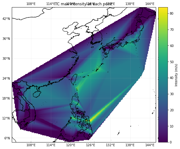
[21]:
tc_cyclone.plot_intensity(event=0)
C:\Users\aleciu\Documents\GitHub\climada_python\climada\util\plot.py:332: UserWarning: Tight layout not applied. The left and right margins cannot be made large enough to accommodate all axes decorations.
  fig.tight_layout()
[21]:
<cartopy.mpl.geoaxes.GeoAxesSubplot at 0x279297a49c8>
[22]:
impf_tc= IFTropCyclone()
impf_tc.set_emanuel_usa()

# add the impact function to an Impact function set
impf_set = ImpactFuncSet()
impf_set.append(impf_tc)
impf_set.check()
2021-03-30 15:19:34,416 - climada.entity.impact_funcs.base - WARNING - For intensity = 0, mdd != 0 or paa != 0. Consider shifting the origin of the intensity scale. In impact.calc the impact is always null at intensity = 0.
[23]:
[haz_type] = impf_set.get_hazard_types()
[haz_id] = impf_set.get_ids()[haz_type]

# Exposures: rename column and assign id
exp_lp.gdf.rename(columns={"if_": "if_" + haz_type}, inplace=True)
exp_lp.gdf['if_' + haz_type] = haz_id
exp_lp.check()
2021-03-30 15:19:34,449 - climada.entity.exposures.base - INFO - category_id not set.
2021-03-30 15:19:34,451 - climada.entity.exposures.base - INFO - cover not set.
2021-03-30 15:19:34,453 - climada.entity.exposures.base - INFO - deductible not set.
2021-03-30 15:19:34,453 - climada.entity.exposures.base - INFO - centr_ not set.
3. Calculate direct, indirect and total impact per sector and country
Let’s now calculate direct, indirect and total impacts. For the direct impact, SupplyChain requires as inputs Hazard, Exposures and ImpactFuncSet. In addition, one may want to specify selected_subsec, which allows the user to either define her own aggregation of sectors by providing a list with the positions of the sectors to aggregate or to use built-in sectors aggregations passing a string being either service, manufacturing, agriculture or mining.
For this tutorial, we will model the service sector, as this sector’s exposure can reasonably be modelled via nighlights and population data, i.e. via LitPop.
3.1 Direct impact
[24]:
supplychain.calc_sector_direct_impact(tc_cyclone, exp_lp, impf_set, selected_subsec='service')
2021-03-30 15:19:34,510 - climada.entity.exposures.base - INFO - meta set to default value {}
2021-03-30 15:19:34,510 - climada.entity.exposures.base - INFO - tag set to default value  File:
 Description:
2021-03-30 15:19:34,513 - climada.entity.exposures.base - INFO - ref_year set to default value 2018
2021-03-30 15:19:34,515 - climada.entity.exposures.base - INFO - value_unit set to default value USD
2021-03-30 15:19:34,517 - climada.entity.exposures.base - INFO - category_id not set.
2021-03-30 15:19:34,518 - climada.entity.exposures.base - INFO - cover not set.
2021-03-30 15:19:34,520 - climada.entity.exposures.base - INFO - deductible not set.
2021-03-30 15:19:34,523 - climada.entity.exposures.base - INFO - centr_ not set.
2021-03-30 15:19:34,528 - climada.entity.exposures.base - INFO - Matching 13993 exposures with 53910 centroids.
2021-03-30 15:19:34,610 - climada.engine.impact - INFO - Calculating damage for 13784 assets (>0) and 65 events.
2021-03-30 15:19:37,499 - climada.entity.exposures.base - INFO - meta set to default value {}
2021-03-30 15:19:37,499 - climada.entity.exposures.base - INFO - tag set to default value  File:
 Description:
2021-03-30 15:19:37,503 - climada.entity.exposures.base - INFO - ref_year set to default value 2018
2021-03-30 15:19:37,503 - climada.entity.exposures.base - INFO - value_unit set to default value USD
2021-03-30 15:19:37,508 - climada.entity.exposures.base - INFO - category_id not set.
2021-03-30 15:19:37,510 - climada.entity.exposures.base - INFO - cover not set.
2021-03-30 15:19:37,510 - climada.entity.exposures.base - INFO - deductible not set.
2021-03-30 15:19:37,512 - climada.entity.exposures.base - INFO - centr_ not set.
2021-03-30 15:19:37,518 - climada.entity.exposures.base - INFO - Matching 1852 exposures with 53910 centroids.
2021-03-30 15:19:37,557 - climada.engine.impact - INFO - Calculating damage for 1849 assets (>0) and 65 events.
2021-03-30 15:19:37,948 - climada.entity.exposures.base - INFO - meta set to default value {}
2021-03-30 15:19:37,948 - climada.entity.exposures.base - INFO - tag set to default value  File:
 Description:
2021-03-30 15:19:37,952 - climada.entity.exposures.base - INFO - ref_year set to default value 2018
2021-03-30 15:19:37,952 - climada.entity.exposures.base - INFO - value_unit set to default value USD
2021-03-30 15:19:37,958 - climada.entity.exposures.base - INFO - category_id not set.
2021-03-30 15:19:37,959 - climada.entity.exposures.base - INFO - cover not set.
2021-03-30 15:19:37,959 - climada.entity.exposures.base - INFO - deductible not set.
2021-03-30 15:19:37,959 - climada.entity.exposures.base - INFO - centr_ not set.
2021-03-30 15:19:37,968 - climada.entity.exposures.base - INFO - Matching 16090 exposures with 53910 centroids.
2021-03-30 15:19:38,093 - climada.engine.impact - INFO - Calculating damage for 16028 assets (>0) and 65 events.
2021-03-30 15:19:38,142 - climada.entity.exposures.base - INFO - meta set to default value {}
2021-03-30 15:19:38,143 - climada.entity.exposures.base - INFO - tag set to default value  File:
 Description:
2021-03-30 15:19:38,145 - climada.entity.exposures.base - INFO - ref_year set to default value 2018
2021-03-30 15:19:38,147 - climada.entity.exposures.base - INFO - value_unit set to default value USD
2021-03-30 15:19:38,149 - climada.entity.exposures.base - INFO - category_id not set.
2021-03-30 15:19:38,151 - climada.entity.exposures.base - INFO - cover not set.
2021-03-30 15:19:38,154 - climada.entity.exposures.base - INFO - deductible not set.
2021-03-30 15:19:38,155 - climada.entity.exposures.base - INFO - centr_ not set.
2021-03-30 15:19:38,162 - climada.entity.exposures.base - INFO - Matching 21975 exposures with 53910 centroids.
2021-03-30 15:19:38,256 - climada.engine.impact - INFO - Calculating damage for 21832 assets (>0) and 65 events.
Let’s see what new attributes the class has got now.
[25]:
supplychain.direct_impact
[25]:
array([[  0.        ,   0.        ,   0.        , ...,  58.55209732,
          3.42504004,   0.        ],
       [  0.        ,   0.        ,   0.        , ..., 470.93561697,
         27.54766205,   0.        ]])
[26]:
supplychain.direct_impact.shape
[26]:
(2, 2464)
All impact matrixes (also those below) provide impacts aggregated over years. They have a number of rows equal to the years being modeled (2 years this time, i.e. 2012-2013) and columns equal to the number of countries times the number of sectors. , i.e. 2464 (see also above).
[27]:
supplychain.direct_aai_agg
[27]:
array([  0.        ,   0.        ,   0.        , ..., 264.74385715,
        15.48635104,   0.        ])
[28]:
supplychain.direct_aai_agg.shape
[28]:
(2464,)
The annual aggregated impact (aai) matrixes provide yearly average impact. They are row vectors with columns equal to the number of countries times the number of sectors, i.e. 2464.
Info for a given country can be accessed as done below:
[29]:
supplychain.direct_aai_agg[supplychain.reg_pos['CHE']]
[29]:
array([0., 0., 0., 0., 0., 0., 0., 0., 0., 0., 0., 0., 0., 0., 0., 0., 0.,
       0., 0., 0., 0., 0., 0., 0., 0., 0., 0., 0., 0., 0., 0., 0., 0., 0.,
       0., 0., 0., 0., 0., 0., 0., 0., 0., 0., 0., 0., 0., 0., 0., 0., 0.,
       0., 0., 0., 0., 0.])
with e.g. CHE, we obviously get zeros, as we are modeling direct impacts in east Asia.
[30]:
supplychain.direct_aai_agg[supplychain.reg_pos['JPN']]
[30]:
array([   0.        ,    0.        ,    0.        ,    0.        ,
          0.        ,    0.        ,    0.        ,    0.        ,
          0.        ,    0.        ,    0.        ,    0.        ,
          0.        ,    0.        ,    0.        ,    0.        ,
          0.        ,    0.        ,    0.        ,    0.        ,
          0.        ,    0.        ,    0.        ,    0.        ,
          0.        ,    0.        ,  965.36489868,  878.15393066,
       2594.28601074,  630.82998657, 1124.37762451,  433.43130493,
        108.08090973,  427.46786499,  153.76459122,  995.37823486,
        274.75501251,  420.40155029,  816.675354  ,  809.9671936 ,
       2277.27154541,  234.72254181,    0.        ,  373.06349945,
          0.        ,    0.        ,   93.46557999,  717.25080872,
       2699.35137939,  565.01576233,  329.95692444,   58.4449482 ,
        256.04863739,  370.85556793,  395.10922241,    0.        ])
for e.g. Japan we instead have direct damages. In order to get all positions of countries undergoing direct damages, one can access the following list:
[31]:
supplychain.reg_dir_imp #note we have two ROW for PHL and VNM
[31]:
['ROW', 'TWN', 'ROW', 'JPN']
and do the following:
[32]:
all_pos = [y for cntry in np.unique(supplychain.reg_dir_imp) for y in supplychain.reg_pos[cntry]]
[33]:
print(supplychain.direct_impact.sum(), supplychain.direct_impact[:, all_pos].sum())
59692.46862970211 59692.46862970211
[34]:
print(supplychain.direct_aai_agg.sum(), supplychain.direct_aai_agg[all_pos].sum())
29846.234314851055 29846.234314851055
i.e., the matrix has non-zero values only at positions corresponding to the modelled countries.
3.2 Indirect impact
For the indirect impact, one can choose the IO modeling approach between Leontief, Ghosh and EEIOA. References are provided below:
[35]:
supplychain.calc_indirect_impact?
Signature: supplychain.calc_indirect_impact(io_approach='ghosh')
Docstring:
Calculate indirect impacts according to the specified input-output
appraoch. This function needs to be run after calc_sector_direct_impact.

Parameters
----------
io_approach : str
    The adopted input-output modeling approach. Possible approaches
    are 'leontief', 'ghosh' and 'eeioa'. Default is 'gosh'.

References
----------
[1] W. W. Leontief, Output, employment, consumption, and investment,
The Quarterly Journal of Economics 58, 1944.
[2] Ghosh, A., Input-Output Approach in an Allocation System,
Economica, New Series, 25, no. 97: 58-64. doi:10.2307/2550694, 1958.
[3] Kitzes, J., An Introduction to Environmentally-Extended Input-Output
Analysis, Resources, 2, 489-503; doi:10.3390/resources2040489, 2013.
File:      c:\users\aleciu\documents\github\climada_python\climada\engine\supplychain.py
Type:      method
Let’s calculate indirect impacts according to the Ghosh method:
[36]:
supplychain.calc_indirect_impact(io_approach='ghosh')
100%|████████████████████████████████████████████████████████████████████████████████████| 2/2 [00:05<00:00, 2.96s/it]
The class now has the indirect impact matrix and vector, with structure equal to those introduced for the direct impact:
[37]:
supplychain.indirect_impact
[37]:
array([[7.5153655e-01, 3.1892043e-02, 4.7066946e-02, ..., 6.7286278e+01,
        3.4250400e+00, 4.2803735e-03],
       [2.1948884e+00, 9.4982922e-02, 1.2662964e-01, ..., 3.7942178e+02,
        2.7547663e+01, 2.1249333e-02]], dtype=float32)
[38]:
supplychain.indirect_impact.shape
[38]:
(2, 2464)
[39]:
supplychain.indirect_aai_agg
[39]:
array([1.4732125e+00, 6.3437484e-02, 8.6848289e-02, ..., 2.2335403e+02,
       1.5486351e+01, 1.2764853e-02], dtype=float32)
If we now check damages for e.g. Switzerland:
[40]:
supplychain.indirect_aai_agg[supplychain.reg_pos['CHE']]
[40]:
array([1.68220580e-01, 9.25031211e-03, 2.74418970e-04, 4.44624610e-02,
       6.71167612e-01, 1.16732985e-01, 1.12433434e-01, 8.17027241e-02,
       6.89174980e-02, 1.35378033e-01, 5.81692576e-01, 2.70589256e+00,
       1.96198016e-01, 1.54878110e-01, 2.06973076e-01, 4.29021597e-01,
       1.89467812e+00, 7.21273184e-01, 7.28916526e-01, 6.06170967e-02,
       1.80502594e-01, 3.23182851e-01, 1.12153739e-01, 1.45547521e+00,
       1.51824072e-01, 0.00000000e+00, 1.18941975e+00, 2.22104624e-01,
       2.23805451e+00, 4.34148878e-01, 1.17412543e+00, 2.86801495e-02,
       4.84273553e-01, 4.27179277e-01, 1.50104269e-01, 3.29186380e-01,
       2.08623365e-01, 0.00000000e+00, 2.89973140e-01, 1.03506613e+00,
       7.41907895e-01, 7.98931241e-01, 0.00000000e+00, 4.80817735e-01,
       5.68698585e-01, 0.00000000e+00, 3.72119516e-01, 0.00000000e+00,
       2.05897242e-01, 4.71446127e-01, 6.04355514e-01, 2.38919139e-01,
       7.35464454e-01, 2.93911517e-01, 0.00000000e+00, 0.00000000e+00],
      dtype=float32)
there are non-zero values, as CH undergoes indirect impacts due to events happening in east Asia.
We can also visualize coefficients, inverse matrix and risk matrix of the selected IO approach:
[41]:
supplychain.io_data
[41]:
{'coefficients': array([[1.55292928e-01, 4.41463292e-03, 2.50902888e-03, ...,
         1.27160543e-04, 0.00000000e+00, 1.66028979e-11],
        [4.62851897e-02, 5.51640205e-02, 1.64963756e-04, ...,
         6.37947051e-06, 0.00000000e+00, 1.15436055e-11],
        [7.32246507e-03, 3.69836880e-06, 7.52862263e-03, ...,
         7.99719510e-06, 0.00000000e+00, 9.63209113e-13],
        ...,
        [5.10453674e-06, 1.68568960e-07, 4.57865355e-07, ...,
         3.88910100e-02, 0.00000000e+00, 1.92610537e-06],
        [1.96250971e-06, 1.90349914e-09, 9.25952381e-09, ...,
         0.00000000e+00, 0.00000000e+00, 0.00000000e+00],
        [0.00000000e+00, 0.00000000e+00, 0.00000000e+00, ...,
         0.00000000e+00, 0.00000000e+00, 0.00000000e+00]], dtype=float32),
 'inverse': array([[1.1956462e+00, 5.6268987e-03, 3.4478118e-03, ..., 1.8672845e-03,
         0.0000000e+00, 1.3596379e-07],
        [7.2838165e-02, 1.0588253e+00, 7.4798276e-04, ..., 1.1149000e-03,
         0.0000000e+00, 1.1273375e-07],
        [1.4281658e-02, 1.1088801e-04, 1.0078237e+00, ..., 5.9475366e-04,
         0.0000000e+00, 6.5748580e-08],
        ...,
        [9.0543799e-05, 5.0534527e-06, 5.3664330e-06, ..., 1.0438221e+00,
         0.0000000e+00, 2.5101926e-06],
        [4.3887998e-05, 1.0840827e-06, 2.1887270e-06, ..., 5.4405088e-04,
         1.0000000e+00, 4.1392159e-08],
        [0.0000000e+00, 0.0000000e+00, 0.0000000e+00, ..., 0.0000000e+00,
         0.0000000e+00, 1.0000000e+00]], dtype=float32),
 'risk_structure': array([[[0.0000000e+00, 0.0000000e+00],
         [0.0000000e+00, 0.0000000e+00],
         [0.0000000e+00, 0.0000000e+00],
         ...,
         [0.0000000e+00, 0.0000000e+00],
         [0.0000000e+00, 0.0000000e+00],
         [0.0000000e+00, 0.0000000e+00]],

        [[0.0000000e+00, 0.0000000e+00],
         [0.0000000e+00, 0.0000000e+00],
         [0.0000000e+00, 0.0000000e+00],
         ...,
         [0.0000000e+00, 0.0000000e+00],
         [0.0000000e+00, 0.0000000e+00],
         [0.0000000e+00, 0.0000000e+00]],

        [[0.0000000e+00, 0.0000000e+00],
         [0.0000000e+00, 0.0000000e+00],
         [0.0000000e+00, 0.0000000e+00],
         ...,
         [0.0000000e+00, 0.0000000e+00],
         [0.0000000e+00, 0.0000000e+00],
         [0.0000000e+00, 0.0000000e+00]],

        ...,

        [[2.6939712e-03, 2.1667661e-02],
         [1.5035659e-04, 1.2093208e-03],
         [1.5966877e-04, 1.2842189e-03],
         ...,
         [3.1057085e+01, 2.4979272e+02],
         [0.0000000e+00, 0.0000000e+00],
         [7.4686359e-05, 6.0070382e-04]],

        [[1.5031816e-04, 1.2090118e-03],
         [3.7130264e-06, 2.9863942e-05],
         [7.4964773e-06, 6.0294311e-05],
         ...,
         [1.8633960e-03, 1.4987330e-02],
         [3.4250400e+00, 2.7547663e+01],
         [1.4176980e-07, 1.1402572e-06]],

        [[0.0000000e+00, 0.0000000e+00],
         [0.0000000e+00, 0.0000000e+00],
         [0.0000000e+00, 0.0000000e+00],
         ...,
         [0.0000000e+00, 0.0000000e+00],
         [0.0000000e+00, 0.0000000e+00],
         [0.0000000e+00, 0.0000000e+00]]], dtype=float32),
 'io_approach': 'ghosh'}
3.3 Total impact
Finally, let’s calculate total impacts, as the sum of both direct and indirect. Therefore, the impact matrixes have the same structure as the direct and indirect matrixes.
[42]:
supplychain.calc_total_impact()
[43]:
supplychain.total_impact
[43]:
array([[7.51536548e-01, 3.18920426e-02, 4.70669456e-02, ...,
        1.25838375e+02, 6.85008004e+00, 4.28037345e-03],
       [2.19488835e+00, 9.49829221e-02, 1.26629636e-01, ...,
        8.50357400e+02, 5.50953248e+01, 2.12493334e-02]])
[44]:
supplychain.total_aai_agg
[44]:
array([1.47321245e+00, 6.34374823e-02, 8.68482906e-02, ...,
       4.88097888e+02, 3.09727024e+01, 1.27648534e-02])
Finally, one can for example visualize total annual average impacts to all Japanese (direct plus indirect) and Swiss (only direct) subsector after TC in East Asia:
[45]:
df_imp = pd.DataFrame(data=np.vstack([supplychain.total_aai_agg[supplychain.reg_pos['CHE']],
                                      supplychain.total_aai_agg[supplychain.reg_pos['JPN']]]),
                      columns=supplychain.sectors,
                      index=['CHE', 'JPN'])
[46]:
df_imp #in M USD
[46]:
| Crop and animal production, hunting and related service activities | Forestry and logging | Fishing and aquaculture | Mining and quarrying | Manufacture of food products, beverages and tobacco products | Manufacture of textiles, wearing apparel and leather products | Manufacture of wood and of products of wood and cork, except furniture; manufacture of articles of straw and plaiting materials | Manufacture of paper and paper products | Printing and reproduction of recorded media | Manufacture of coke and refined petroleum products | ... | Scientific research and development | Advertising and market research | Other professional, scientific and technical activities; veterinary activities | Administrative and support service activities | Public administration and defence; compulsory social security | Education | Human health and social work activities | Other service activities | Activities of households as employers; undifferentiated goods- and services-producing activities of households for own use | Activities of extraterritorial organizations and bodies | |
|---|---|---|---|---|---|---|---|---|---|---|---|---|---|---|---|---|---|---|---|---|---|
| CHE | 0.168221 | 0.009250 | 0.000274 | 0.044462 | 0.671168 | 0.116733 | 0.112433 | 0.081703 | 0.068917 | 0.135378 | ... | 0.372120 | 0.000000 | 0.205897 | 0.471446 | 0.604356 | 0.238919 | 0.735464 | 0.293912 | 0.000000 | 0.0 |
| JPN | 94.852016 | 8.924538 | 15.782462 | 39.295603 | 423.523209 | 64.728909 | 23.186090 | 119.893147 | 62.801826 | 53.429245 | ... | 187.867998 | 1149.998154 | 5108.261841 | 1049.191330 | 1184.859177 | 226.233683 | 1048.544487 | 865.901283 | 594.775421 | 0.0 |
2 rows × 56 columns
[ ]: