Exposures class#
What is an exposure?#
Exposure describes the set of assets, people, livelihoods, infrastructures, etc. within an area of interest in terms of their geographic location, their value etc.; in brief - everything potentially exposed to hazards.
What options does CLIMADA offer for me to create an exposure?#
CLIMADA has an Exposures class for this purpuse. An Exposures instance can be filled with your own data, or loaded from available default sources implemented through some Exposures-type classes from CLIMADA.
If you have your own data, they can be provided in the formats of a pandas.DataFrame, a geopandas.GeoDataFrame or simply an Excel file.
If you didn’t collect your own data, exposures can be generated on the fly using CLIMADA’s LitPop, BlackMarble or OpenStreetMap modules. See the respective tutorials to learn what exactly they contain and how to use them.
What does an exposure look like in CLIMADA?#
An exposure is represented in the class Exposures, which contains a geopandas GeoDataFrame that is accessible through the Exposures.data attribute.
A “geometry” column is initialized in the GeoDataFrame of the Exposures object, other columns are optional at first but some have to be present or make a difference when it comes to do calculations.
Apart from these special columns the data frame may contain additional columns, they will simply be ignored in the context of CLIMADA.
The full list of meaningful columns is this:
Column |
Data Type |
Description |
Meaningful in |
Optional |
|---|---|---|---|---|
|
Point |
the geometry column of the |
centroids assignment |
- |
|
float |
a value for each exposure |
impact calculation |
✔* |
|
int |
impact functions ids for hazard types. |
impact calculation |
✔* |
|
int |
centroids index for hazard type. |
impact calculation |
✔* |
|
float |
deductible value for each exposure. |
impact calculation |
✔ |
|
float |
cover value for each exposure. |
impact calculation |
✔ |
|
int |
region id (e.g. country ISO code) for each exposure |
aggregation |
✔ |
|
int |
category id (e.g. building code) for each exposure |
aggregation |
✔ |
*) an Exposures object is valid without such a column, but it’s required for impact calculation
Apart from data the Exposures object has the following attributes and properties:
Attributes |
Data Type |
Description |
|---|---|---|
|
str |
describing origin and content of the exposures data |
|
int |
reference year |
|
str |
unit of the exposures’ values |
Properties |
Data Type |
Description |
|---|---|---|
|
numpy.array[Point] |
array of geometry values |
|
pyproj.CRS |
coordinate reference system, see GeoDataFrame.crs |
|
numpy.array[float] |
array of latitude values |
|
numpy.array[float] |
array of longitude values |
|
numpy.array[int] |
array of regeion_id values |
|
numpy.array[int] |
array of category_id values |
|
numpy.array[float] |
array of cover values |
|
numpy.array[float] |
array of cover values |
Defining exposures from your own data#
The essential structure of an exposure is similar, irrespective of the data type you choose to provide: As mentioned in the introduction, the key variables to be provided are latitudes, longitudes and values of your exposed assets.
While not mandatory, but very useful to provide for the impact calculation at later stages: the impact function id (see impf_* in the table above).
The following examples will walk you through how to specifiy those four variables, and demonstrate the use of a few more optional parameters on the go.
Exposures from plain data#
import numpy as np
from climada.entity import Exposures

latitude = [1, 2, 3] * 3
longitude = [4] * 3 + [5] * 3 + [6] * 3
exp_arr = Exposures(
    lat=latitude,  # list or array
    lon=longitude,  # instead of lat and lon one can provide an array of Points through the geometry argument
    value=np.random.random_sample(len(latitude)),  # a list or an array of floats
    value_unit="CHF",
    crs="EPSG:7316",  # different formats are possible
    description="random values in a square",
    data={
        "region_id": 1,
        "impf_": range(len(latitude)),
    },  # data can also be an array or a data frame
)
print(exp_arr)
description: random values in a square
ref_year: 2018
value_unit: CHF
crs: EPSG:7316
data: (9 entries)
   region_id  impf_             geometry     value
0          1      0  POINT (4.000 1.000)  0.035321
1          1      1  POINT (4.000 2.000)  0.570256
2          1      2  POINT (4.000 3.000)  0.927632
3          1      3  POINT (5.000 1.000)  0.805402
4          1      4  POINT (5.000 2.000)  0.236179
5          1      5  POINT (5.000 3.000)  0.848296
6          1      6  POINT (6.000 1.000)  0.520281
7          1      7  POINT (6.000 2.000)  0.036442
8          1      8  POINT (6.000 3.000)  0.780934
Exposures from a pandas DataFrame#
In case you are unfamiliar with the data structure, check out the pandas DataFrame documentation.
import numpy as np
from pandas import DataFrame
from climada.entity import Exposures

# Fill a pandas DataFrame with the 3 mandatory variables (latitude, longitude, value) for a number of assets (10'000).
# We will do this with random dummy data for purely illustrative reasons:
exp_df = DataFrame()
n_exp = 100 * 100
# provide value
exp_df["value"] = np.random.random_sample(n_exp)
# provide latitude and longitude
lat, lon = np.mgrid[
    15 : 35 : complex(0, np.sqrt(n_exp)), 20 : 40 : complex(0, np.sqrt(n_exp))
]
exp_df["latitude"] = lat.flatten()
exp_df["longitude"] = lon.flatten()
# For each exposure entry, specify which impact function should be taken for which hazard type.
# In this case, we only specify the IDs for tropical cyclone (TC); here, each exposure entry will be treated with
# the same impact function: the one that has ID '1':
# Of course, this will only be relevant at later steps during impact calculations.
exp_df["impf_TC"] = np.ones(n_exp, int)
exp_df
| value | latitude | longitude | impf_TC | |
|---|---|---|---|---|
| 0 | 0.533764 | 15.0 | 20.000000 | 1 |
| 1 | 0.995993 | 15.0 | 20.202020 | 1 |
| 2 | 0.603523 | 15.0 | 20.404040 | 1 |
| 3 | 0.754253 | 15.0 | 20.606061 | 1 |
| 4 | 0.305066 | 15.0 | 20.808081 | 1 |
| ... | ... | ... | ... | ... |
| 9995 | 0.482416 | 35.0 | 39.191919 | 1 |
| 9996 | 0.069044 | 35.0 | 39.393939 | 1 |
| 9997 | 0.116560 | 35.0 | 39.595960 | 1 |
| 9998 | 0.239856 | 35.0 | 39.797980 | 1 |
| 9999 | 0.099568 | 35.0 | 40.000000 | 1 |
10000 rows × 4 columns
# Generate Exposures from the pandas DataFrame. This step converts the DataFrame into
# a CLIMADA Exposures instance!
exp = Exposures(exp_df)
print(f"exp has the type: {type(exp)}")
print(f"and contains a GeoDataFrame exp.gdf: {type(exp.gdf)}\n")
exp has the type: <class 'climada.entity.exposures.base.Exposures'>
and contains a GeoDataFrame exp.gdf: <class 'geopandas.geodataframe.GeoDataFrame'>
# let's have a look at the Exposures instance we created!
print(exp)
description: None
ref_year: 2018
value_unit: USD
crs: EPSG:4326
data: (10000 entries)
         value  impf_TC                   geometry
0     0.533764        1  POINT (20.00000 15.00000)
1     0.995993        1  POINT (20.20202 15.00000)
2     0.603523        1  POINT (20.40404 15.00000)
3     0.754253        1  POINT (20.60606 15.00000)
9996  0.069044        1  POINT (39.39394 35.00000)
9997  0.116560        1  POINT (39.59596 35.00000)
9998  0.239856        1  POINT (39.79798 35.00000)
9999  0.099568        1  POINT (40.00000 35.00000)
Exposures from a geopandas GeoDataFrame#
In case you are unfamiliar with with data structure, check out the geopandas GeoDataFrame documentation.
The main difference to the example above (pandas DataFrame) is that, while previously, we provided latitudes and longitudes which were then converted to a geometry GeoSeries using the set_geometry_points method, GeoDataFrames alread come with a defined geometry GeoSeries. In this case, we take the geometry info and use the set_lat_lon method to explicitly provide latitudes and longitudes.
This example focuses on data with POINT geometry, but in principle, other geometry types (such as POLYGON and MULTIPOLYGON) would work as well.
import numpy as np
import geopandas as gpd
from climada.entity import Exposures

# Read spatial info from an external file into GeoDataFrame
world = gpd.read_file(gpd.datasets.get_path("naturalearth_cities"))
C:\Users\me\AppData\Local\Temp\ipykernel_31104\2272990317.py:6: FutureWarning: The geopandas.dataset module is deprecated and will be removed in GeoPandas 1.0. You can get the original 'naturalearth_cities' data from https://www.naturalearthdata.com/downloads/110m-cultural-vectors/.
  world = gpd.read_file(gpd.datasets.get_path('naturalearth_cities'))
# Generate Exposures: value, latitude and longitude for each exposure entry.
world["value"] = np.arange(n_exp)
# Convert GeoDataFrame into Exposure instance
exp_gpd = Exposures(world)
print(exp_gpd)
description: None
ref_year: 2018
value_unit: USD
crs: EPSG:4326
data: (243 entries)
             name     value                     geometry
0    Vatican City  0.876947    POINT (12.45339 41.90328)
1      San Marino  0.895454    POINT (12.44177 43.93610)
2           Vaduz  0.373366     POINT (9.51667 47.13372)
3         Lobamba  0.422729   POINT (31.20000 -26.46667)
239     São Paulo  0.913955  POINT (-46.62697 -23.55673)
240        Sydney  0.514479  POINT (151.21255 -33.87137)
241     Singapore  0.830635    POINT (103.85387 1.29498)
242     Hong Kong  0.764571   POINT (114.18306 22.30693)
# For each exposure entry, specify which impact function should be taken for which hazard type.
# In this case, we only specify the IDs for tropical cyclone (TC); here, each exposure entry will be treated with
# the same impact function: the one that has ID '1':
# Of course, this will only be relevant at later steps during impact calculations.
exp_gpd.data["impf_TC"] = np.ones(world.shape[0], int)
print(exp_gpd)
description: None
ref_year: 2018
value_unit: USD
crs: EPSG:4326
data: (243 entries)
             name     value                     geometry  impf_TC
0    Vatican City  0.876947    POINT (12.45339 41.90328)        1
1      San Marino  0.895454    POINT (12.44177 43.93610)        1
2           Vaduz  0.373366     POINT (9.51667 47.13372)        1
3         Lobamba  0.422729   POINT (31.20000 -26.46667)        1
239     São Paulo  0.913955  POINT (-46.62697 -23.55673)        1
240        Sydney  0.514479  POINT (151.21255 -33.87137)        1
241     Singapore  0.830635    POINT (103.85387 1.29498)        1
242     Hong Kong  0.764571   POINT (114.18306 22.30693)        1
The fact that Exposures is built around a geopandas.GeoDataFrame offers all the useful functionalities that come with the package. The following examples showcase only a few of those.
# Example 1: extract data in a region: latitudes between -5 and 5
sel_exp = exp_gpd.copy()  # to keep the original exp_gpd Exposures data
sel_exp.data = sel_exp.data.cx[:, -5:5]

print("\n" + "sel_exp contains a subset of the original data")
sel_exp.data
sel_exp contains a subset of the original data
| name | value | impf_TC | geometry | |
|---|---|---|---|---|
| 11 | Tarawa | 0.107688 | 1 | POINT (173.01757 1.33819) |
| 15 | Kigali | 0.218687 | 1 | POINT (30.05859 -1.95164) |
| 17 | Juba | 0.763743 | 1 | POINT (31.58003 4.82998) |
| 31 | Putrajaya | 0.533607 | 1 | POINT (101.69504 2.93252) |
| 37 | Bujumbura | 0.127881 | 1 | POINT (29.36001 -3.37609) |
| 58 | Kampala | 0.079019 | 1 | POINT (32.58138 0.31860) |
| 75 | Mogadishu | 0.696766 | 1 | POINT (45.36473 2.06863) |
| 88 | Quito | 0.212070 | 1 | POINT (-78.50200 -0.21304) |
| 93 | Malabo | 0.088459 | 1 | POINT (8.78328 3.75002) |
| 99 | Libreville | 0.929139 | 1 | POINT (9.45796 0.38539) |
| 108 | Brazzaville | 0.795766 | 1 | POINT (15.28274 -4.25724) |
| 113 | Bandar Seri Begawan | 0.655856 | 1 | POINT (114.93328 4.88333) |
| 116 | Bangui | 0.398002 | 1 | POINT (18.55829 4.36664) |
| 117 | Yaoundé | 0.240599 | 1 | POINT (11.51470 3.86865) |
| 134 | Victoria | 0.956208 | 1 | POINT (55.44999 -4.61663) |
| 135 | São Tomé | 0.726704 | 1 | POINT (6.72965 0.33747) |
| 138 | Malé | 0.996017 | 1 | POINT (73.50890 4.17204) |
| 158 | Kuala Lumpur | 0.880473 | 1 | POINT (101.68870 3.13980) |
| 201 | Kinshasa | 0.074387 | 1 | POINT (15.31303 -4.32778) |
| 228 | Nairobi | 0.297170 | 1 | POINT (36.81471 -1.28140) |
| 230 | Bogota | 0.420891 | 1 | POINT (-74.08529 4.59837) |
| 241 | Singapore | 0.830635 | 1 | POINT (103.85387 1.29498) |
# Example 2: extract data in a polygon
from shapely.geometry import Polygon

sel_polygon = exp_gpd.copy()  # to keep the original exp_gpd Exposures data

poly = Polygon([(0, -10), (0, 10), (10, 5)])
sel_polygon.data = sel_polygon.gdf[sel_polygon.gdf.intersects(poly)]

# Let's have a look. Again, the sub-selection is a GeoDataFrame!
print("\n" + "sel_exp contains a subset of the original data")
sel_polygon.data
sel_exp contains a subset of the original data
| name | value | impf_TC | geometry | |
|---|---|---|---|---|
| 36 | Porto-Novo | 0.573619 | 1 | POINT (2.61663 6.48331) |
| 46 | Lomé | 0.176892 | 1 | POINT (1.22081 6.13388) |
| 93 | Malabo | 0.088459 | 1 | POINT (8.78328 3.75002) |
| 123 | Cotonou | 0.441703 | 1 | POINT (2.40435 6.36298) |
| 135 | São Tomé | 0.726704 | 1 | POINT (6.72965 0.33747) |
| 225 | Lagos | 0.990135 | 1 | POINT (3.38959 6.44521) |
# Example 3: change coordinate reference system
# use help to see more options: help(sel_exp.to_crs)
sel_polygon.to_crs(epsg=3395, inplace=True)
print("\n" + "the crs has changed to " + str(sel_polygon.crs))
print(
    "the values for latitude and longitude are now according to the new coordinate system: "
)
sel_polygon.data
the crs has changed to EPSG:3395
the values for latitude and longitude are now according to the new coordinate system:
| name | value | impf_TC | geometry | |
|---|---|---|---|---|
| 36 | Porto-Novo | 0.573619 | 1 | POINT (291281.418 718442.692) |
| 46 | Lomé | 0.176892 | 1 | POINT (135900.092 679566.331) |
| 93 | Malabo | 0.088459 | 1 | POINT (977749.979 414955.553) |
| 123 | Cotonou | 0.441703 | 1 | POINT (267651.551 705052.049) |
| 135 | São Tomé | 0.726704 | 1 | POINT (749141.190 37315.322) |
| 225 | Lagos | 0.990135 | 1 | POINT (377326.898 714202.107) |
# Example 4: concatenate exposures
exp_all = Exposures.concat([sel_polygon, sel_exp.to_crs(epsg=3395)])

# the output is of type Exposures
print("exp_all type and number of rows:", type(exp_all), exp_all.gdf.shape[0])
print("number of unique rows:", exp_all.gdf.drop_duplicates().shape[0])

# NaNs will appear in the missing values
exp_all.data.tail()
exp_all type and number of rows: <class 'climada.entity.exposures.base.Exposures'> 28
number of unique rows: 26
| name | value | impf_TC | geometry | |
|---|---|---|---|---|
| 23 | Kuala Lumpur | 0.880473 | 1 | POINT (11319934.225 347356.996) |
| 24 | Kinshasa | 0.074387 | 1 | POINT (1704638.257 -479002.730) |
| 25 | Nairobi | 0.297170 | 1 | POINT (4098194.882 -141701.948) |
| 26 | Bogota | 0.420891 | 1 | POINT (-8247136.736 509015.405) |
| 27 | Singapore | 0.830635 | 1 | POINT (11560960.460 143203.754) |
Exposures of any file type supported by Geopandas and Pandas#
Geopandas can read almost any vector-based spatial data format including ESRI shapefile, GeoJSON files and more, see readers geopandas. Pandas supports formats such as csv, html or sql; see readers pandas. Using the corresponding readers, DataFrame and GeoDataFrame can be filled and provided to Exposures following the previous examples.
Exposures from an excel file#
If you manually collect exposure data, Excel may be your preferred option.
In this case, it is easiest if you format your data according to the structure provided in the template climada_python/climada/data/system/entity_template.xlsx, in the sheet assets.
import pandas as pd
from climada.util.constants import ENT_TEMPLATE_XLS
from climada.entity import Exposures

# Read your Excel file into a pandas DataFrame (we will use the template example for this demonstration):
file_name = ENT_TEMPLATE_XLS
exp_templ = pd.read_excel(file_name)

# Let's have a look at the data:
print("exp_templ is a DataFrame:", str(type(exp_templ)))
print("exp_templ looks like:")
exp_templ.head()
exp_templ is a DataFrame: <class 'pandas.core.frame.DataFrame'>
exp_templ looks like:
| latitude | longitude | value | deductible | cover | region_id | category_id | impf_TC | centr_TC | impf_FL | centr_FL | |
|---|---|---|---|---|---|---|---|---|---|---|---|
| 0 | 26.933899 | -80.128799 | 1.392750e+10 | 0 | 1.392750e+10 | 1 | 1 | 1 | 1 | 1 | 1 |
| 1 | 26.957203 | -80.098284 | 1.259606e+10 | 0 | 1.259606e+10 | 1 | 1 | 1 | 2 | 1 | 2 |
| 2 | 26.783846 | -80.748947 | 1.259606e+10 | 0 | 1.259606e+10 | 1 | 1 | 1 | 3 | 1 | 3 |
| 3 | 26.645524 | -80.550704 | 1.259606e+10 | 0 | 1.259606e+10 | 1 | 1 | 1 | 4 | 1 | 4 |
| 4 | 26.897796 | -80.596929 | 1.259606e+10 | 0 | 1.259606e+10 | 1 | 1 | 1 | 5 | 1 | 5 |
As we can see, the general structure is the same as always: the exposure has latitude, longitude and value columns. Further, this example specified several impact function ids: some for Tropical Cyclones (impf_TC), and some for Floods (impf_FL). It also provides some meta-info (region_id, category_id) and insurance info relevant to the impact calculation in later steps (cover, deductible).
# Generate an Exposures instance from the dataframe.
exp_templ = Exposures(exp_templ)
print("\n" + "exp_templ is now an Exposures:", exp_templ)
exp_templ is now an Exposures: description: None
ref_year: 2018
value_unit: USD
crs: EPSG:4326
data: (24 entries)
           value  deductible         cover  region_id  category_id  impf_TC  \
0   1.392750e+10           0  1.392750e+10          1            1        1
1   1.259606e+10           0  1.259606e+10          1            1        1
2   1.259606e+10           0  1.259606e+10          1            1        1
3   1.259606e+10           0  1.259606e+10          1            1        1
20  1.259760e+10           0  1.259760e+10          1            1        1
21  1.281454e+10           0  1.281454e+10          1            1        1
22  1.262176e+10           0  1.262176e+10          1            1        1
23  1.259754e+10           0  1.259754e+10          1            1        1

    centr_TC  impf_FL  centr_FL                    geometry
0          1        1         1  POINT (-80.12880 26.93390)
1          2        1         2  POINT (-80.09828 26.95720)
2          3        1         3  POINT (-80.74895 26.78385)
3          4        1         4  POINT (-80.55070 26.64552)
20        21        1        21  POINT (-80.06858 26.71255)
21        22        1        22  POINT (-80.09070 26.66490)
22        23        1        23  POINT (-80.12540 26.66470)
23        24        1        24  POINT (-80.15140 26.66315)
Exposures from a raster file#
Last but not least, you may have your exposure data stored in a raster file. Raster data may be read in from any file-type supported by rasterio.
from rasterio.windows import Window
from climada.util.constants import HAZ_DEMO_FL
from climada.entity import Exposures

# We take an example with a dummy raster file (HAZ_DEMO_FL), running the method set_from_raster directly loads the
# necessary info from the file into an Exposures instance.
exp_raster = Exposures.from_raster(HAZ_DEMO_FL, window=Window(10, 20, 50, 60))
# There are several keyword argument options that come with the set_from_raster method (such as
# specifying a window, if not the entire file should be read, or a bounding box. Check them out.
2024-10-04 17:19:03,632 - climada.util.coordinates - INFO - Reading C:\Users\me\climada\demo\data\SC22000_VE__M1.grd.gz
exp_raster.derive_raster()
2024-10-04 17:19:03,725 - climada.util.coordinates - INFO - Raster from resolution 0.009000000000000341 to 0.009000000000000341.
{'crs': <Geographic 2D CRS: EPSG:4326>
 Name: WGS 84
 Axis Info [ellipsoidal]:
 - Lat[north]: Geodetic latitude (degree)
 - Lon[east]: Geodetic longitude (degree)
 Area of Use:
 - name: World.
 - bounds: (-180.0, -90.0, 180.0, 90.0)
 Datum: World Geodetic System 1984 ensemble
 - Ellipsoid: WGS 84
 - Prime Meridian: Greenwich,
 'height': 60,
 'width': 50,
 'transform': Affine(0.009000000000000341, 0.0, -69.2471495969998,
        0.0, -0.009000000000000341, 10.248220966978932)}
Loading CLIMADA-generated exposure files or generating new ones#
In case you already have a CLIMADA-generated file containing Exposures info, you can of course load it back into memory. Most likely, the data format will either be of .hdf5 or of .mat.
In case you neither have your own data, nor a CLIMADA-generated file, you can also create an exposure on the fly using one of the three CLIMADA-internal exposure generators: LitPop, BlackMarble or OpenStreetMap modules. The latter three are extensively described in their own, linked, tutorials.
# read  generated with the Python version with from_hdf5()
# note: for .mat data, use the method from_mat() analogously.
from climada.util.constants import EXP_DEMO_H5

exp_hdf5 = Exposures.from_hdf5(EXP_DEMO_H5)
print(exp_hdf5)
2024-10-04 17:19:04,888 - climada.entity.exposures.base - INFO - Reading C:\Users\me\climada\demo\data\exp_demo_today.h5
description: None
ref_year: 2016
value_unit: USD
crs: EPSG:4326
data: (50 entries)
           value  impf_TC  deductible         cover  category_id  region_id  \
0   1.392750e+10        1         0.0  1.392750e+10            1        1.0
1   1.259606e+10        1         0.0  1.259606e+10            1        1.0
2   1.259606e+10        1         0.0  1.259606e+10            1        1.0
3   1.259606e+10        1         0.0  1.259606e+10            1        1.0
46  1.264524e+10        1         0.0  1.264524e+10            1        1.0
47  1.281438e+10        1         0.0  1.281438e+10            1        1.0
48  1.260291e+10        1         0.0  1.260291e+10            1        1.0
49  1.262482e+10        1         0.0  1.262482e+10            1        1.0

                      geometry
0   POINT (-80.12880 26.93390)
1   POINT (-80.09828 26.95720)
2   POINT (-80.74895 26.78385)
3   POINT (-80.55070 26.64552)
46  POINT (-80.11640 26.34907)
47  POINT (-80.08385 26.34635)
48  POINT (-80.24130 26.34802)
49  POINT (-80.15886 26.34796)
c:\Users\me\miniconda3\envs\climada_env\Lib\pickle.py:1718: UserWarning: Unpickling a shapely <2.0 geometry object. Please save the pickle again; shapely 2.1 will not have this compatibility.
  setstate(state)
Visualize Exposures#
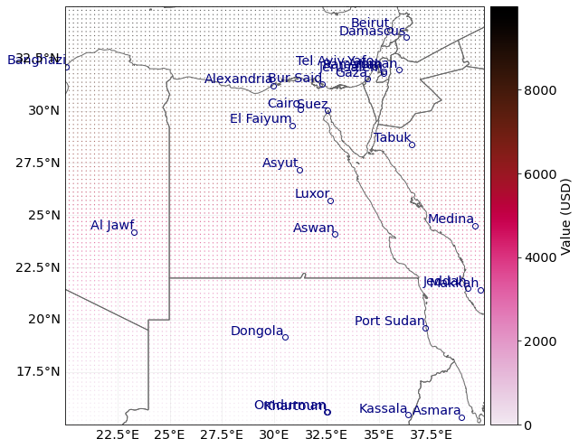
The method plot_hexbin() uses cartopy and matplotlib’s hexbin function to represent the exposures values as 2d bins over a map. Configure your plot by fixing the different inputs of the method or by modifying the returned matplotlib figure and axes.
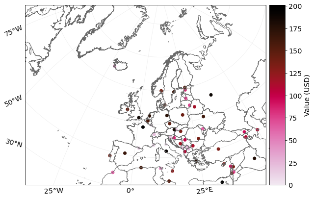
The method plot_scatter() uses cartopy and matplotlib’s scatter function to represent the points values over a 2d map. As usal, it returns the figure and axes, which can be modify aftwerwards.
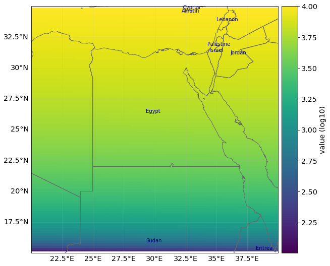
The method plot_raster() rasterizes the points into the given resolution. Use the save_tiff option to save the resulting tiff file and the res_rasteroption to re-set the raster’s resolution.
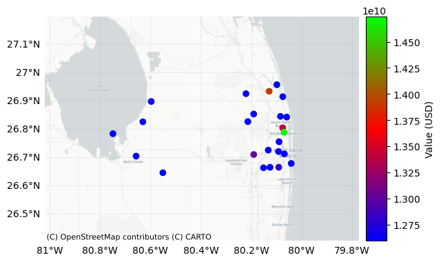
Finally, the method plot_basemap() plots the scatter points over a satellite image using contextily library.
# Example 1: plot_hexbin method
print("Plotting exp_df.")
axs = exp.plot_hexbin();

# further methods to check out:
# axs.set_xlim(15, 45) to modify x-axis borders, axs.set_ylim(10, 40) to modify y-axis borders
# further keyword arguments to play around with: pop_name, buffer, gridsize, ...
Plotting exp_df.
# Example 2: plot_scatter method

exp_gpd.to_crs("epsg:3035", inplace=True)
exp_gpd.plot_scatter(pop_name=False);
<GeoAxesSubplot:>
# Example 3: plot_raster method
from climada.util.plot import add_cntry_names  # use climada's plotting utilities

ax = exp.plot_raster()
# plot with same resolution as data
add_cntry_names(
    ax,
    [
        exp.gdf["longitude"].min(),
        exp.gdf["longitude"].max(),
        exp.gdf["latitude"].min(),
        exp.gdf["latitude"].max(),
    ],
)

# use keyword argument save_tiff='filepath.tiff' to save the corresponding raster in tiff format
# use keyword argument raster_res='desired number' to change resolution of the raster.
2021-06-04 17:07:42,654 - climada.util.coordinates - INFO - Raster from resolution 0.20202020202019355 to 0.20202020202019355.
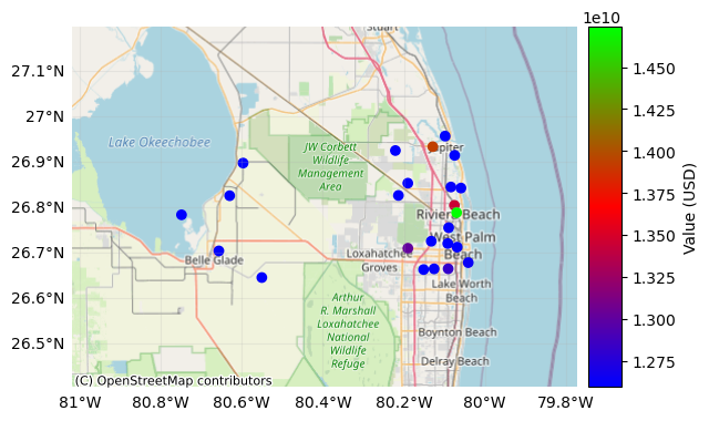
# Example 4: plot_basemap method
import contextily as ctx

# select the background image from the available ctx.providers
ax = exp_templ.plot_basemap(buffer=30000, cmap="brg")
# using Positron from CartoDB
ax = exp_templ.plot_basemap(
    buffer=30000,
    cmap="brg",
    url=ctx.providers.OpenStreetMap.Mapnik,  # Using OpenStreetmap,
    zoom=9,
);  # select the zoom level of the map, affects the font size of labelled objects
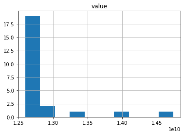
Since Exposures is a GeoDataFrame, any function for visualization from geopandas can be used. Check making maps and examples gallery.
# other visualization types
exp_templ.gdf.hist(column="value");
array([[<AxesSubplot:title={'center':'value'}>]], dtype=object)
Write (Save) Exposures#
Exposures can be saved in any format available for GeoDataFrame (see fiona.supported_drivers) and DataFrame (pandas IO tools). Take into account that in many of these formats the metadata (e.g. variables ref_year and value_unit) will not be saved. Use instead the format hdf5 provided by Exposures methods write_hdf5() and from_hdf5() to handle all the data.
import fiona

fiona.supported_drivers
from climada import CONFIG

results = CONFIG.local_data.save_dir.dir()

# DataFrame save to csv format. geometry writen as string, metadata not saved!
exp_templ.gdf.to_csv(results.joinpath("exp_templ.csv"), sep="\t")
# write as hdf5 file
exp_templ.write_hdf5(results.joinpath("exp_temp.h5"))
Optionally use climada’s save option to save it in pickle format. This allows fast to quickly restore the object in its current state and take up your work right were you left it the next time. Note however, that pickle has a transient format and is not suitable for storing data persistently.
# save in pickle format
from climada.util.save import save

# this generates a results folder in the current path and stores the output there
save("exp_templ.pkl.p", exp_templ)  # creates results folder and stores there