How to use polygons or lines as exposure#
Introduction#
Exposure in CLIMADA are usually represented as individual points or a raster of points.
See Exposures tutorial to learn how to fill and use exposures.
In this tutorial we show you how to run the impact calculation chain if you have polygons or lines to start with.
The approach provides an all-in-one method for impact calculation: calc_geom_impact
It features three sub-steps, for which the current util module lines_polys_handler also provides separate functions:
Disaggregation of line and polygon data into point exposure:
Interpolate geometries to points to fit in an
Exposureinstance;Disaggregate the respective geometry values to the point values
Perform the impact calculation in CLIMADA with the point exposure
Aggregate the calculated point
Impactback to an impact instance for the initial polygons or lines
Note: Polygons or lines can be useful to represent specific types of exposures such as infrastructures (e.g. roads) or landuse types (e.g. crops, forests). In CLIMADA, it is possible to retrieve such specific exposure types using OpenStreetMap data. Please refer to the associated tutorial to learn how to do so.
Quick example#
Get example polygons (provinces), lines (rails), points exposure for the Netherlands, and create one single Exposures. Get demo winter storm hazard and a corresponding impact function.
from climada.util.api_client import Client
import climada.util.lines_polys_handler as u_lp
from climada.entity.impact_funcs import ImpactFuncSet
from climada.entity.impact_funcs.storm_europe import ImpfStormEurope
from climada.entity import Exposures

HAZ = Client().get_hazard("storm_europe", name="test_haz_WS_nl", status="test_dataset")

EXP_POLY = Client().get_exposures(
    "base", name="test_polygon_exp", status="test_dataset"
)
EXP_LINE = Client().get_exposures("base", name="test_line_exp", status="test_dataset")
EXP_POINT = Client().get_exposures("base", name="test_point_exp", status="test_dataset")

EXP_MIX = Exposures.concat([EXP_POLY, EXP_LINE, EXP_POINT])

IMPF = ImpfStormEurope.from_welker()
IMPF_SET = ImpactFuncSet([IMPF])
Compute the impact in one line.
# disaggregate in the same CRS as the exposures are defined (here degrees), resolution 1degree
# divide values on points
# aggregate by summing

impact = u_lp.calc_geom_impact(
    exp=EXP_MIX,
    impf_set=IMPF_SET,
    haz=HAZ,
    res=0.2,
    to_meters=False,
    disagg_met=u_lp.DisaggMethod.DIV,
    disagg_val=None,
    agg_met=u_lp.AggMethod.SUM,
)
2022-06-24 13:16:15,277 - climada.entity.exposures.base - INFO - Setting latitude and longitude attributes.
2022-06-24 13:16:15,284 - climada.entity.exposures.base - INFO - Matching 183 exposures with 9944 centroids.
2022-06-24 13:16:15,285 - climada.util.coordinates - INFO - No exact centroid match found. Reprojecting coordinates to nearest neighbor closer than the threshold = 100
2022-06-24 13:16:15,295 - climada.engine.impact - INFO - Exposures matching centroids found in centr_WS
2022-06-24 13:16:15,296 - climada.engine.impact - INFO - Calculating damage for 182 assets (>0) and 2 events.
/Users/ckropf/Documents/Climada/climada_python/climada/util/lines_polys_handler.py:931: UserWarning: Geometry is in a geographic CRS. Results from 'length' are likely incorrect. Use 'GeoSeries.to_crs()' to re-project geometries to a projected CRS before this operation.

  line_lengths = gdf_lines.length
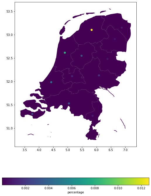
u_lp.plot_eai_exp_geom(impact);
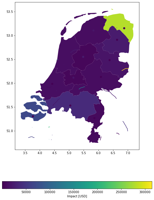
# disaggregate in meters
# same value for each point, fixed to 1 (allows to get percentages of affected surface/distance)
# aggregate by summing

impact = u_lp.calc_geom_impact(
    exp=EXP_MIX,
    impf_set=IMPF_SET,
    haz=HAZ,
    res=1000,
    to_meters=True,
    disagg_met=u_lp.DisaggMethod.FIX,
    disagg_val=1.0,
    agg_met=u_lp.AggMethod.SUM,
);
2022-06-24 13:16:17,387 - climada.entity.exposures.base - INFO - Setting latitude and longitude attributes.
2022-06-24 13:16:18,069 - climada.entity.exposures.base - INFO - Matching 37357 exposures with 9944 centroids.
2022-06-24 13:16:18,073 - climada.util.coordinates - INFO - No exact centroid match found. Reprojecting coordinates to nearest neighbor closer than the threshold = 100
2022-06-24 13:16:18,114 - climada.engine.impact - INFO - Exposures matching centroids found in centr_WS
2022-06-24 13:16:18,117 - climada.engine.impact - INFO - Calculating damage for 37357 assets (>0) and 2 events.
import matplotlib.pyplot as plt

ax = u_lp.plot_eai_exp_geom(
    impact, legend_kwds={"label": "percentage", "orientation": "horizontal"}
)
Polygons#
Polygons or shapes are a common geographical representation of countries, states etc. as for example in NaturalEarth. Map data, as for example buildings, etc. obtained from openstreetmap (see tutorial here), also frequently come as (multi-)polygons. Here we want to show you how to deal with exposure information as polygons.
Load data#
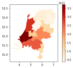
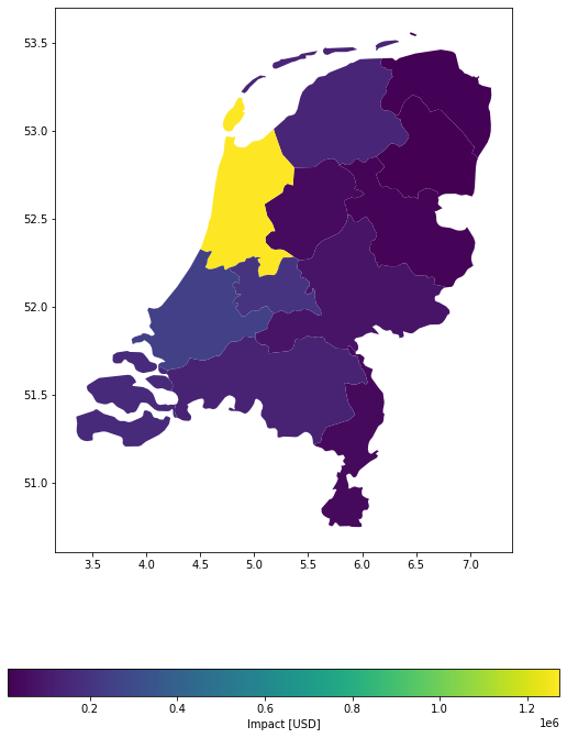
Lets assume we have the following data given. The polygons of the admin-1 regions of the Netherlands and an exposure value each, which we gather in a geodataframe. We want to know the Impact of Lothar on each admin-1 region.
In this tutorial, we shall see how to compute impacts for exposures defined on shapely geometries (polygons and/or lines). The basic principle is to disaggregate the geometries to a raster of points, compute the impact per points, and then re-aggregate. To do so, several methods are available. Here is a brief overview.
# Imports
import geopandas as gpd
import pandas as pd
from pathlib import Path

from climada.entity import Exposures
from climada.entity.impact_funcs.storm_europe import ImpfStormEurope
from climada.entity.impact_funcs import ImpactFuncSet
from climada.engine import ImpactCalc
from climada.hazard.storm_europe import StormEurope
import climada.util.lines_polys_handler as u_lp
from climada.util.constants import DEMO_DIR, WS_DEMO_NC
def gdf_poly():
    from cartopy.io import shapereader
    from climada_petals.entity.exposures.black_marble import country_iso_geom

    # open the file containing the Netherlands admin-1 polygons
    shp_file = shapereader.natural_earth(
        resolution="10m", category="cultural", name="admin_0_countries"
    )
    shp_file = shapereader.Reader(shp_file)

    # extract the NL polygons
    prov_names = {
        "Netherlands": [
            "Groningen",
            "Drenthe",
            "Overijssel",
            "Gelderland",
            "Limburg",
            "Zeeland",
            "Noord-Brabant",
            "Zuid-Holland",
            "Noord-Holland",
            "Friesland",
            "Flevoland",
            "Utrecht",
        ]
    }
    polygon_Netherlands, polygons_prov_NL = country_iso_geom(prov_names, shp_file)
    prov_geom_NL = {
        prov: geom
        for prov, geom in zip(
            list(prov_names.values())[0], list(polygons_prov_NL.values())[0]
        )
    }

    # assign a value to each admin-1 area (assumption 100'000 USD per inhabitant)
    population_prov_NL = {
        "Drenthe": 493449,
        "Flevoland": 422202,
        "Friesland": 649988,
        "Gelderland": 2084478,
        "Groningen": 585881,
        "Limburg": 1118223,
        "Noord-Brabant": 2562566,
        "Noord-Holland": 2877909,
        "Overijssel": 1162215,
        "Zuid-Holland": 3705625,
        "Utrecht": 1353596,
        "Zeeland": 383689,
    }
    value_prov_NL = {
        n: 100000 * population_prov_NL[n] for n in population_prov_NL.keys()
    }

    # combine into GeoDataFrame and add a coordinate reference system to it:
    df1 = pd.DataFrame.from_dict(
        population_prov_NL, orient="index", columns=["population"]
    ).join(pd.DataFrame.from_dict(value_prov_NL, orient="index", columns=["value"]))
    df1["geometry"] = [prov_geom_NL[prov] for prov in df1.index]
    gdf_polys = gpd.GeoDataFrame(df1)
    gdf_polys = gdf_polys.set_crs(epsg=4326)
    return gdf_polys
exp_nl_poly = Exposures(gdf_poly())
exp_nl_poly.gdf["impf_WS"] = 1
exp_nl_poly.gdf.head()
| population | value | geometry | impf_WS | |
|---|---|---|---|---|
| Drenthe | 493449 | 49344900000 | POLYGON ((7.07215 52.84132, 7.06198 52.82401, ... | 1 |
| Flevoland | 422202 | 42220200000 | POLYGON ((5.74046 52.83874, 5.75012 52.83507, ... | 1 |
| Friesland | 649988 | 64998800000 | MULTIPOLYGON (((5.17977 53.00899, 5.27947 53.0... | 1 |
| Gelderland | 2084478 | 208447800000 | POLYGON ((6.77158 52.10879, 6.76587 52.10840, ... | 1 |
| Groningen | 585881 | 58588100000 | MULTIPOLYGON (((7.19459 53.24502, 7.19747 53.2... | 1 |
# take a look
exp_nl_poly.gdf.plot("value", legend=True, cmap="OrRd")
<AxesSubplot:>
# define hazard
storms = StormEurope.from_footprints(WS_DEMO_NC)
# define impact function
impf = ImpfStormEurope.from_welker()
impf_set = ImpactFuncSet([impf])
2022-06-24 13:16:20,039 - climada.hazard.storm_europe - INFO - Constructing centroids from /Users/ckropf/climada/demo/data/fp_lothar_crop-test.nc
2022-06-24 13:16:20,124 - climada.hazard.centroids.centr - INFO - Convert centroids to GeoSeries of Point shapes.
/Users/ckropf/Documents/Climada/climada_python/climada/hazard/centroids/centr.py:822: UserWarning: Geometry is in a geographic CRS. Results from 'buffer' are likely incorrect. Use 'GeoSeries.to_crs()' to re-project geometries to a projected CRS before this operation.

  xy_pixels = self.geometry.buffer(res / 2).envelope
2022-06-24 13:16:22,004 - climada.hazard.storm_europe - INFO - Commencing to iterate over netCDF files.
Compute polygon impacts - all in one#
All in one: The main method calc_geom_impact provides several disaggregation keywords, specifiying
the target resolution (
res),the method on how to distribute the values of the original geometries onto the newly generated interpolated points (
disagg_met)the source (and number) of the value to be distributed (
disagg_val).the aggregation method (
agg_met)
disagg_met can be either fixed (FIX), replicating the original shape’s value onto all points, or divided evenly (DIV), in which case the value is divided equally onto all new points.
disagg_val can either be taken directly from the exposure gdf’s value column (None) or be indicated here explicitly (float). Resolution can be given in the gdf’s original (mostly degrees lat/lon) format, or in metres. agg_met can currently be only (SUM) were the value is summed over all points in the geometry.
Polygons can also be disaggregated on a given fixed grid, see example below
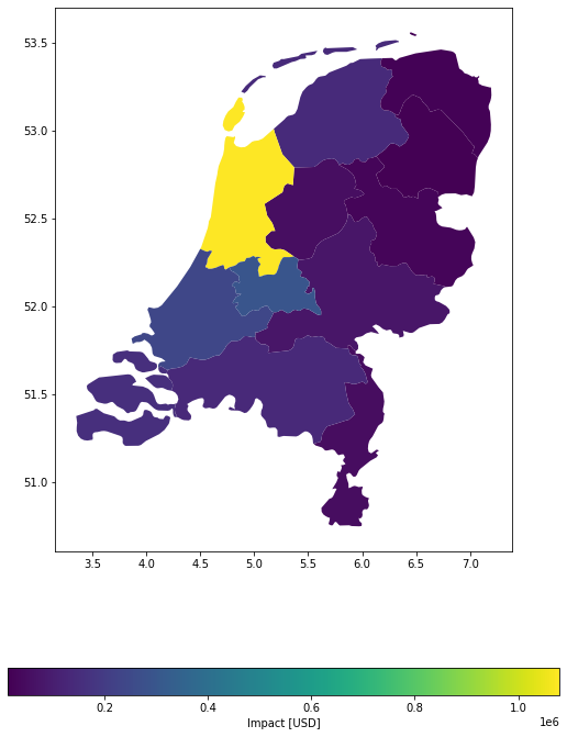
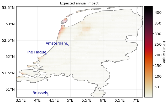
Example 1: Target resolution in degrees lat/lon, equal (average) distribution of values from exposure gdf among points.
imp_deg = u_lp.calc_geom_impact(
    exp=exp_nl_poly,
    impf_set=impf_set,
    haz=storms,
    res=0.005,
    disagg_met=u_lp.DisaggMethod.DIV,
    disagg_val=None,
    agg_met=u_lp.AggMethod.SUM,
)
2022-06-24 13:16:30,535 - climada.entity.exposures.base - INFO - Setting latitude and longitude attributes.
2022-06-24 13:16:33,946 - climada.entity.exposures.base - INFO - Matching 195323 exposures with 9944 centroids.
2022-06-24 13:16:33,950 - climada.util.coordinates - INFO - No exact centroid match found. Reprojecting coordinates to nearest neighbor closer than the threshold = 100
2022-06-24 13:16:34,140 - climada.engine.impact - INFO - Exposures matching centroids found in centr_WS
2022-06-24 13:16:34,144 - climada.engine.impact - INFO - Calculating damage for 195323 assets (>0) and 2 events.
u_lp.plot_eai_exp_geom(imp_deg);

Example 2: Target resolution in metres, equal (divide) distribution of values from exposure gdf among points.
imp_m = u_lp.calc_geom_impact(
    exp=exp_nl_poly,
    impf_set=impf_set,
    haz=storms,
    res=500,
    to_meters=True,
    disagg_met=u_lp.DisaggMethod.DIV,
    disagg_val=None,
    agg_met=u_lp.AggMethod.SUM,
)
2022-06-24 13:16:41,366 - climada.entity.exposures.base - INFO - Setting latitude and longitude attributes.
2022-06-24 13:16:44,164 - climada.entity.exposures.base - INFO - Matching 148369 exposures with 9944 centroids.
2022-06-24 13:16:44,168 - climada.util.coordinates - INFO - No exact centroid match found. Reprojecting coordinates to nearest neighbor closer than the threshold = 100
2022-06-24 13:16:44,387 - climada.engine.impact - INFO - Exposures matching centroids found in centr_WS
2022-06-24 13:16:44,390 - climada.engine.impact - INFO - Calculating damage for 148369 assets (>0) and 2 events.
u_lp.plot_eai_exp_geom(imp_m);
For this specific case, both disaggregation methods provide a relatively similar result, given the chosen numbers:
(imp_deg.eai_exp - imp_m.eai_exp) / imp_deg.eai_exp
array([ 0.00614586, -0.01079377,  0.00021355,  0.00140608,  0.0038771 ,
       -0.0066888 , -0.00171755,  0.00741871, -0.00107029,  0.00424221,
       -0.01838225,  0.01811858])
Example 3: Target predefined grid, equal (divide) distribution of values from exposure gdf among points.
# regular grid from exposures bounds
import climada.util.coordinates as u_coord

res = 0.1
(_, _, xmax, ymax) = exp_nl_poly.gdf.geometry.bounds.max()
(xmin, ymin, _, _) = exp_nl_poly.gdf.geometry.bounds.min()
bounds = (xmin, ymin, xmax, ymax)
height, width, trafo = u_coord.pts_to_raster_meta(bounds, (res, res))
x_grid, y_grid = u_coord.raster_to_meshgrid(trafo, width, height)
imp_g = u_lp.calc_grid_impact(
    exp=exp_nl_poly,
    impf_set=impf_set,
    haz=storms,
    grid=(x_grid, y_grid),
    disagg_met=u_lp.DisaggMethod.DIV,
    disagg_val=None,
    agg_met=u_lp.AggMethod.SUM,
)
2022-06-24 13:16:45,086 - climada.entity.exposures.base - INFO - Setting latitude and longitude attributes.
2022-06-24 13:16:45,100 - climada.entity.exposures.base - INFO - Matching 486 exposures with 9944 centroids.
2022-06-24 13:16:45,102 - climada.util.coordinates - INFO - No exact centroid match found. Reprojecting coordinates to nearest neighbor closer than the threshold = 100
2022-06-24 13:16:45,110 - climada.engine.impact - INFO - Exposures matching centroids found in centr_WS
2022-06-24 13:16:45,111 - climada.engine.impact - INFO - Calculating damage for 486 assets (>0) and 2 events.
u_lp.plot_eai_exp_geom(imp_g);
Compute polygon impacts - step by step#
Step 1: Disaggregate polygon exposures to points. It is useful to do this separately, when the discretized exposure is used several times, for example, to compute with different hazards.
Several disaggregation methods can be used as shown below:
# Disaggregate exposure to 10'000 metre grid, each point gets average value within polygon.
exp_pnt = u_lp.exp_geom_to_pnt(
    exp_nl_poly,
    res=10000,
    to_meters=True,
    disagg_met=u_lp.DisaggMethod.DIV,
    disagg_val=None,
)
exp_pnt.gdf.head()
2022-06-24 13:16:45,445 - climada.entity.exposures.base - INFO - Setting latitude and longitude attributes.
| population | value | geometry_orig | impf_WS | geometry | latitude | longitude | ||
|---|---|---|---|---|---|---|---|---|
| Drenthe | 0 | 493449 | 2.056038e+09 | POLYGON ((7.07215 52.84132, 7.06198 52.82401, ... | 1 | POINT (6.21931 52.75939) | 52.759394 | 6.219308 |
| 1 | 493449 | 2.056038e+09 | POLYGON ((7.07215 52.84132, 7.06198 52.82401, ... | 1 | POINT (6.30914 52.75939) | 52.759394 | 6.309139 | |
| 2 | 493449 | 2.056038e+09 | POLYGON ((7.07215 52.84132, 7.06198 52.82401, ... | 1 | POINT (6.39897 52.75939) | 52.759394 | 6.398971 | |
| 3 | 493449 | 2.056038e+09 | POLYGON ((7.07215 52.84132, 7.06198 52.82401, ... | 1 | POINT (6.48880 52.75939) | 52.759394 | 6.488802 | |
| 4 | 493449 | 2.056038e+09 | POLYGON ((7.07215 52.84132, 7.06198 52.82401, ... | 1 | POINT (6.57863 52.75939) | 52.759394 | 6.578634 |
# Disaggregate exposure to 0.1° grid, no value disaggregation specified --> replicate initial value
exp_pnt2 = u_lp.exp_geom_to_pnt(
    exp_nl_poly,
    res=0.1,
    to_meters=False,
    disagg_met=u_lp.DisaggMethod.FIX,
    disagg_val=None,
)
exp_pnt2.gdf.head()
2022-06-24 13:16:45,516 - climada.entity.exposures.base - INFO - Setting latitude and longitude attributes.
| population | value | geometry_orig | impf_WS | geometry | latitude | longitude | ||
|---|---|---|---|---|---|---|---|---|
| Drenthe | 0 | 493449 | 49344900000 | POLYGON ((7.07215 52.84132, 7.06198 52.82401, ... | 1 | POINT (6.22948 52.71147) | 52.711466 | 6.229476 |
| 1 | 493449 | 49344900000 | POLYGON ((7.07215 52.84132, 7.06198 52.82401, ... | 1 | POINT (6.32948 52.71147) | 52.711466 | 6.329476 | |
| 2 | 493449 | 49344900000 | POLYGON ((7.07215 52.84132, 7.06198 52.82401, ... | 1 | POINT (6.42948 52.71147) | 52.711466 | 6.429476 | |
| 3 | 493449 | 49344900000 | POLYGON ((7.07215 52.84132, 7.06198 52.82401, ... | 1 | POINT (6.52948 52.71147) | 52.711466 | 6.529476 | |
| 4 | 493449 | 49344900000 | POLYGON ((7.07215 52.84132, 7.06198 52.82401, ... | 1 | POINT (6.62948 52.71147) | 52.711466 | 6.629476 |
# Disaggregate exposure to 1'000 metre grid, each point gets value corresponding to
# its representative area (1'000^2).
exp_pnt3 = u_lp.exp_geom_to_pnt(
    exp_nl_poly,
    res=1000,
    to_meters=True,
    disagg_met=u_lp.DisaggMethod.FIX,
    disagg_val=10e6,
)
exp_pnt3.gdf.head()
2022-06-24 13:16:47,258 - climada.entity.exposures.base - INFO - Setting latitude and longitude attributes.
| population | value | geometry_orig | impf_WS | geometry | latitude | longitude | ||
|---|---|---|---|---|---|---|---|---|
| Drenthe | 0 | 493449 | 10000000.0 | POLYGON ((7.07215 52.84132, 7.06198 52.82401, ... | 1 | POINT (6.38100 52.62624) | 52.626236 | 6.381005 |
| 1 | 493449 | 10000000.0 | POLYGON ((7.07215 52.84132, 7.06198 52.82401, ... | 1 | POINT (6.38999 52.62624) | 52.626236 | 6.389988 | |
| 2 | 493449 | 10000000.0 | POLYGON ((7.07215 52.84132, 7.06198 52.82401, ... | 1 | POINT (6.39897 52.62624) | 52.626236 | 6.398971 | |
| 3 | 493449 | 10000000.0 | POLYGON ((7.07215 52.84132, 7.06198 52.82401, ... | 1 | POINT (6.40795 52.62624) | 52.626236 | 6.407954 | |
| 4 | 493449 | 10000000.0 | POLYGON ((7.07215 52.84132, 7.06198 52.82401, ... | 1 | POINT (6.41694 52.62624) | 52.626236 | 6.416937 |
# Disaggregate exposure to 1'000 metre grid, each point gets value corresponding to 1
# After dissagregation, each point has a value equal to the percentage of area of the polygon
exp_pnt4 = u_lp.exp_geom_to_pnt(
    exp_nl_poly,
    res=1000,
    to_meters=True,
    disagg_met=u_lp.DisaggMethod.DIV,
    disagg_val=1,
)
exp_pnt4.gdf.tail()
2022-06-24 13:16:49,929 - climada.entity.exposures.base - INFO - Setting latitude and longitude attributes.
| population | value | geometry_orig | impf_WS | geometry | latitude | longitude | ||
|---|---|---|---|---|---|---|---|---|
| Zeeland | 1897 | 383689 | 0.000526 | MULTIPOLYGON (((3.45388 51.23563, 3.42194 51.2... | 1 | POINT (3.92434 51.73813) | 51.738126 | 3.924336 |
| 1898 | 383689 | 0.000526 | MULTIPOLYGON (((3.45388 51.23563, 3.42194 51.2... | 1 | POINT (3.93332 51.73813) | 51.738126 | 3.933320 | |
| 1899 | 383689 | 0.000526 | MULTIPOLYGON (((3.45388 51.23563, 3.42194 51.2... | 1 | POINT (3.94230 51.73813) | 51.738126 | 3.942303 | |
| 1900 | 383689 | 0.000526 | MULTIPOLYGON (((3.45388 51.23563, 3.42194 51.2... | 1 | POINT (3.95129 51.73813) | 51.738126 | 3.951286 | |
| 1901 | 383689 | 0.000526 | MULTIPOLYGON (((3.45388 51.23563, 3.42194 51.2... | 1 | POINT (3.96027 51.73813) | 51.738126 | 3.960269 |
# disaggregate on pre-defined grid
# regular grid from exposures bounds
import climada.util.coordinates as u_coord

res = 0.1
(_, _, xmax, ymax) = exp_nl_poly.gdf.geometry.bounds.max()
(xmin, ymin, _, _) = exp_nl_poly.gdf.geometry.bounds.min()
bounds = (xmin, ymin, xmax, ymax)
height, width, trafo = u_coord.pts_to_raster_meta(bounds, (res, res))
x_grid, y_grid = u_coord.raster_to_meshgrid(trafo, width, height)
exp_pnt5 = u_lp.exp_geom_to_grid(
    exp_nl_poly, grid=(x_grid, y_grid), disagg_met=u_lp.DisaggMethod.DIV, disagg_val=1
)
exp_pnt5.gdf.tail()
2022-06-24 13:16:50,765 - climada.entity.exposures.base - INFO - Setting latitude and longitude attributes.
| population | value | geometry_orig | impf_WS | geometry | latitude | longitude | ||
|---|---|---|---|---|---|---|---|---|
| Zeeland | 17 | 383689 | 0.045455 | MULTIPOLYGON (((3.45388 51.23563, 3.42194 51.2... | 1 | POINT (3.84941 51.54755) | 51.54755 | 3.849415 |
| 18 | 383689 | 0.045455 | MULTIPOLYGON (((3.45388 51.23563, 3.42194 51.2... | 1 | POINT (4.14941 51.54755) | 51.54755 | 4.149415 | |
| 19 | 383689 | 0.045455 | MULTIPOLYGON (((3.45388 51.23563, 3.42194 51.2... | 1 | POINT (3.94941 51.64755) | 51.64755 | 3.949415 | |
| 20 | 383689 | 0.045455 | MULTIPOLYGON (((3.45388 51.23563, 3.42194 51.2... | 1 | POINT (4.04941 51.64755) | 51.64755 | 4.049415 | |
| 21 | 383689 | 0.045455 | MULTIPOLYGON (((3.45388 51.23563, 3.42194 51.2... | 1 | POINT (4.14941 51.64755) | 51.64755 | 4.149415 |
Step 2: Calculate point impacts & re-aggregate them afterwards
# Point-impact
imp_pnt = ImpactCalc(exp_pnt3, impf_set, hazard=storms).impact(save_mat=True)

# Aggregated impact (Note that you need to pass the gdf and not the exposures)
imp_geom = u_lp.impact_pnt_agg(imp_pnt, exp_pnt3.gdf, agg_met=u_lp.AggMethod.SUM)
2022-06-24 13:16:50,793 - climada.entity.exposures.base - INFO - Matching 37082 exposures with 9944 centroids.
2022-06-24 13:16:50,796 - climada.util.coordinates - INFO - No exact centroid match found. Reprojecting coordinates to nearest neighbor closer than the threshold = 100
2022-06-24 13:16:50,929 - climada.engine.impact - INFO - Calculating damage for 37082 assets (>0) and 2 events.
# Plot point-impacts and aggregated impacts
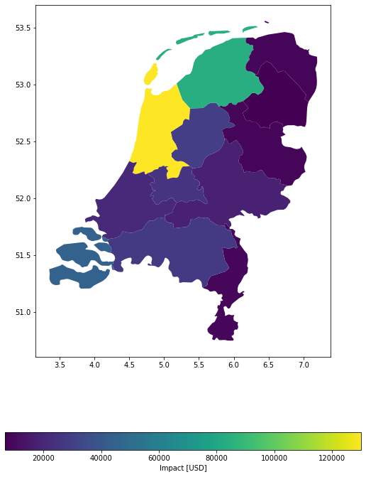
imp_pnt.plot_hexbin_eai_exposure()
u_lp.plot_eai_exp_geom(imp_geom);
2022-06-24 13:16:51,002 - climada.util.plot - WARNING - Error parsing coordinate system 'epsg:4326'. Using projection PlateCarree in plot.
Aggregated impact, in detail
# aggregate impact matrix
mat_agg = u_lp._aggregate_impact_mat(imp_pnt, exp_pnt3.gdf, agg_met=u_lp.AggMethod.SUM)

eai_exp = u_lp.eai_exp_from_mat(imp_mat=mat_agg, freq=imp_pnt.frequency)
at_event = u_lp.at_event_from_mat(imp_mat=mat_agg)
aai_agg = u_lp.aai_agg_from_at_event(at_event=at_event, freq=imp_pnt.frequency)
eai_exp
array([  6753.45186608,  28953.21638482,  84171.28903387,  18014.15630989,
         8561.18507994,   8986.13653385,  27446.46387061, 130145.29903078,
         8362.17243334,  20822.87844894,  25495.46296087,  45121.14833362])
at_event
array([4321211.03400214, 219950.4291506 ])
aai_agg
412832.8602866131
Lines#
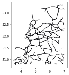
Lines are common geographical representation of transport infrastructure like streets, train tracks or powerlines etc. Here we will play it through for the case of winter storm Lothar’s impact on the Dutch Railway System:
Loading Data#
Note: Hazard and impact functions data have been loaded above.
def gdf_lines():
    gdf_lines = gpd.read_file(Path(DEMO_DIR, "nl_rails.gpkg"))
    gdf_lines = gdf_lines.to_crs(epsg=4326)
    return gdf_lines
exp_nl_lines = Exposures(gdf_lines())
exp_nl_lines.gdf["impf_WS"] = 1
exp_nl_lines.gdf["value"] = 1
exp_nl_lines.gdf.head()
| distance | geometry | impf_WS | value | |
|---|---|---|---|---|
| 0 | 9414.978692 | LINESTRING (6.08850 50.87940, 6.08960 50.87850... | 1 | 1 |
| 1 | 10397.965112 | LINESTRING (6.17673 51.35530, 6.17577 51.35410... | 1 | 1 |
| 2 | 26350.219724 | LINESTRING (5.68096 51.25040, 5.68422 51.25020... | 1 | 1 |
| 3 | 40665.249638 | LINESTRING (5.68096 51.25040, 5.67711 51.25030... | 1 | 1 |
| 4 | 8297.689753 | LINESTRING (5.70374 50.85490, 5.70531 50.84990... | 1 | 1 |
exp_nl_lines.gdf.plot("value", cmap="inferno");
Calculating line impacts - all in one#
Example 1: Disaggregate values evenly among road segments; split in points with 0.005 degree distances.
imp_deg = u_lp.calc_geom_impact(
    exp=exp_nl_lines,
    impf_set=impf_set,
    haz=storms,
    res=0.005,
    disagg_met=u_lp.DisaggMethod.DIV,
    disagg_val=None,
    agg_met=u_lp.AggMethod.SUM,
)
/Users/ckropf/Documents/Climada/climada_python/climada/util/lines_polys_handler.py:931: UserWarning: Geometry is in a geographic CRS. Results from 'length' are likely incorrect. Use 'GeoSeries.to_crs()' to re-project geometries to a projected CRS before this operation.

  line_lengths = gdf_lines.length
2022-06-24 13:16:59,608 - climada.entity.exposures.base - INFO - Setting latitude and longitude attributes.
2022-06-24 13:16:59,787 - climada.entity.exposures.base - INFO - Matching 10175 exposures with 9944 centroids.
2022-06-24 13:16:59,789 - climada.util.coordinates - INFO - No exact centroid match found. Reprojecting coordinates to nearest neighbor closer than the threshold = 100
2022-06-24 13:16:59,805 - climada.engine.impact - INFO - Exposures matching centroids found in centr_WS
2022-06-24 13:16:59,806 - climada.engine.impact - INFO - Calculating damage for 10175 assets (>0) and 2 events.
u_lp.plot_eai_exp_geom(imp_deg);

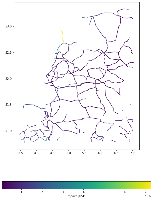
Example 2: Disaggregate values evenly among road segments; split in points with 500 m distances.
imp_m = u_lp.calc_geom_impact(
    exp=exp_nl_lines,
    impf_set=impf_set,
    haz=storms,
    res=500,
    to_meters=True,
    disagg_met=u_lp.DisaggMethod.DIV,
    disagg_val=None,
    agg_met=u_lp.AggMethod.SUM,
)
2022-06-24 13:17:00,670 - climada.entity.exposures.base - INFO - Setting latitude and longitude attributes.
2022-06-24 13:17:00,827 - climada.entity.exposures.base - INFO - Matching 8399 exposures with 9944 centroids.
2022-06-24 13:17:00,828 - climada.util.coordinates - INFO - No exact centroid match found. Reprojecting coordinates to nearest neighbor closer than the threshold = 100
2022-06-24 13:17:00,843 - climada.engine.impact - INFO - Exposures matching centroids found in centr_WS
2022-06-24 13:17:00,845 - climada.engine.impact - INFO - Calculating damage for 8399 assets (>0) and 2 events.
u_lp.plot_eai_exp_geom(imp_m);
import numpy as np

diff = np.max((imp_deg.eai_exp - imp_m.eai_exp) / imp_deg.eai_exp)
print(
    f"The largest relative different between degrees and meters impact in this example is {diff}"
)
The largest relative different between degrees and meters impact in this example is 0.09803913811822067
Calculating line impacts - step by step#
Step 1: As in the polygon example above, there are several methods to disaggregate line exposures into point exposures, of which several are shown here:
# 0.1° distance between points, average value disaggregation
exp_pnt = u_lp.exp_geom_to_pnt(
    exp_nl_lines,
    res=0.1,
    to_meters=False,
    disagg_met=u_lp.DisaggMethod.DIV,
    disagg_val=None,
)
exp_pnt.gdf.head()
2022-06-24 13:17:01,409 - climada.entity.exposures.base - INFO - Setting latitude and longitude attributes.
/Users/ckropf/Documents/Climada/climada_python/climada/util/lines_polys_handler.py:931: UserWarning: Geometry is in a geographic CRS. Results from 'length' are likely incorrect. Use 'GeoSeries.to_crs()' to re-project geometries to a projected CRS before this operation.

  line_lengths = gdf_lines.length
| distance | geometry_orig | impf_WS | value | geometry | latitude | longitude | ||
|---|---|---|---|---|---|---|---|---|
| 0 | 0 | 9414.978692 | LINESTRING (6.08850 50.87940, 6.08960 50.87850... | 1 | 0.500000 | POINT (6.08850 50.87940) | 50.879400 | 6.088500 |
| 1 | 9414.978692 | LINESTRING (6.08850 50.87940, 6.08960 50.87850... | 1 | 0.500000 | POINT (6.06079 50.80030) | 50.800300 | 6.060790 | |
| 1 | 0 | 10397.965112 | LINESTRING (6.17673 51.35530, 6.17577 51.35410... | 1 | 0.333333 | POINT (6.17673 51.35530) | 51.355300 | 6.176730 |
| 1 | 10397.965112 | LINESTRING (6.17673 51.35530, 6.17577 51.35410... | 1 | 0.333333 | POINT (6.12632 51.32440) | 51.324399 | 6.126323 | |
| 2 | 10397.965112 | LINESTRING (6.17673 51.35530, 6.17577 51.35410... | 1 | 0.333333 | POINT (6.08167 51.28460) | 51.284600 | 6.081670 |
# 1000m distance between points, no value disaggregation
exp_pnt2 = u_lp.exp_geom_to_pnt(
    exp_nl_lines,
    res=1000,
    to_meters=True,
    disagg_met=u_lp.DisaggMethod.FIX,
    disagg_val=None,
)
exp_pnt2.gdf.head()
2022-06-24 13:17:01,876 - climada.entity.exposures.base - INFO - Setting latitude and longitude attributes.
| distance | geometry_orig | impf_WS | value | geometry | latitude | longitude | ||
|---|---|---|---|---|---|---|---|---|
| 0 | 0 | 9414.978692 | LINESTRING (6.08850 50.87940, 6.08960 50.87850... | 1 | 1 | POINT (6.08850 50.87940) | 50.879400 | 6.088500 |
| 1 | 9414.978692 | LINESTRING (6.08850 50.87940, 6.08960 50.87850... | 1 | 1 | POINT (6.09416 50.87275) | 50.872755 | 6.094165 | |
| 2 | 9414.978692 | LINESTRING (6.08850 50.87940, 6.08960 50.87850... | 1 | 1 | POINT (6.09161 50.86410) | 50.864105 | 6.091608 | |
| 3 | 9414.978692 | LINESTRING (6.08850 50.87940, 6.08960 50.87850... | 1 | 1 | POINT (6.08744 50.85590) | 50.855902 | 6.087435 | |
| 4 | 9414.978692 | LINESTRING (6.08850 50.87940, 6.08960 50.87850... | 1 | 1 | POINT (6.08326 50.84770) | 50.847699 | 6.083263 |
# 1000m distance between points, equal value disaggregation
exp_pnt3 = u_lp.exp_geom_to_pnt(
    exp_nl_lines,
    res=1000,
    to_meters=True,
    disagg_met=u_lp.DisaggMethod.DIV,
    disagg_val=None,
)
exp_pnt3.gdf.head()
2022-06-24 13:17:02,436 - climada.entity.exposures.base - INFO - Setting latitude and longitude attributes.
| distance | geometry_orig | impf_WS | value | geometry | latitude | longitude | ||
|---|---|---|---|---|---|---|---|---|
| 0 | 0 | 9414.978692 | LINESTRING (6.08850 50.87940, 6.08960 50.87850... | 1 | 0.090909 | POINT (6.08850 50.87940) | 50.879400 | 6.088500 |
| 1 | 9414.978692 | LINESTRING (6.08850 50.87940, 6.08960 50.87850... | 1 | 0.090909 | POINT (6.09416 50.87275) | 50.872755 | 6.094165 | |
| 2 | 9414.978692 | LINESTRING (6.08850 50.87940, 6.08960 50.87850... | 1 | 0.090909 | POINT (6.09161 50.86410) | 50.864105 | 6.091608 | |
| 3 | 9414.978692 | LINESTRING (6.08850 50.87940, 6.08960 50.87850... | 1 | 0.090909 | POINT (6.08744 50.85590) | 50.855902 | 6.087435 | |
| 4 | 9414.978692 | LINESTRING (6.08850 50.87940, 6.08960 50.87850... | 1 | 0.090909 | POINT (6.08326 50.84770) | 50.847699 | 6.083263 |
# 1000m distance between points, disaggregation of value according to representative distance
exp_pnt4 = u_lp.exp_geom_to_pnt(
    exp_nl_lines,
    res=1000,
    to_meters=True,
    disagg_met=u_lp.DisaggMethod.FIX,
    disagg_val=1000,
)
exp_pnt4.gdf.head()
2022-06-24 13:17:03,116 - climada.entity.exposures.base - INFO - Setting latitude and longitude attributes.
| distance | geometry_orig | impf_WS | value | geometry | latitude | longitude | ||
|---|---|---|---|---|---|---|---|---|
| 0 | 0 | 9414.978692 | LINESTRING (6.08850 50.87940, 6.08960 50.87850... | 1 | 1000 | POINT (6.08850 50.87940) | 50.879400 | 6.088500 |
| 1 | 9414.978692 | LINESTRING (6.08850 50.87940, 6.08960 50.87850... | 1 | 1000 | POINT (6.09416 50.87275) | 50.872755 | 6.094165 | |
| 2 | 9414.978692 | LINESTRING (6.08850 50.87940, 6.08960 50.87850... | 1 | 1000 | POINT (6.09161 50.86410) | 50.864105 | 6.091608 | |
| 3 | 9414.978692 | LINESTRING (6.08850 50.87940, 6.08960 50.87850... | 1 | 1000 | POINT (6.08744 50.85590) | 50.855902 | 6.087435 | |
| 4 | 9414.978692 | LINESTRING (6.08850 50.87940, 6.08960 50.87850... | 1 | 1000 | POINT (6.08326 50.84770) | 50.847699 | 6.083263 |
Step 2 & 3: The procedure is analogous to the example provided above for polygons.